P71
文章目录
- 4.1 李群与李代数基础
- 4.1.3 李代数的定义
- 4.1.4 李代数 so(3)
- 4.1.5 李代数 se(3)
- 4.2 指数与对数映射
- 4.2.1 SO(3)上的指数映射
- 罗德里格斯公式推导
- 4.2.2 SE(3) 上的指数映射
- SO(3),SE(3),so(3),se(3)的对应关系
- 4.3 李代数求导与扰动模型
- 4.3.2 SO(3)上的李代数求导
- 4.3.3 李代数求导
- 4.3.4 扰动模型(左乘)【更简单 的导数计算模型】
- 4.3.5 SE(3)上的李代数求导
- 4.4 Sophus应用 【Code】
- 4.4.2 评估轨迹的误差 【Code】
- 4.5 相似变换群 与 李代数
- 习题
- 题1
- 题2
- 题4
- √ 题5
- √ 题6
- 6.2 SE(3)伴随性质
- √ 题7
- √ 题8
- LaTex

什么样的相机位姿 最符合 当前观测数据。
求解最优的 R , t \bm{R, t} R,t, 使得误差最小化。
4.1 李群与李代数基础

群: 只有一个(良好的)运算的集合。


封结幺逆 、 丰俭由你

李群: 具有连续(光滑)性质的群。


在 t = 0 附近,旋转矩阵可以由 e x p ( ϕ 0 ˆ t ) exp(\phi_0\^{}t) exp(ϕ0ˆt)计算得到
4.1.3 李代数的定义

李代数 描述了李群的局部性质
- 单位元 附近的正切空间。
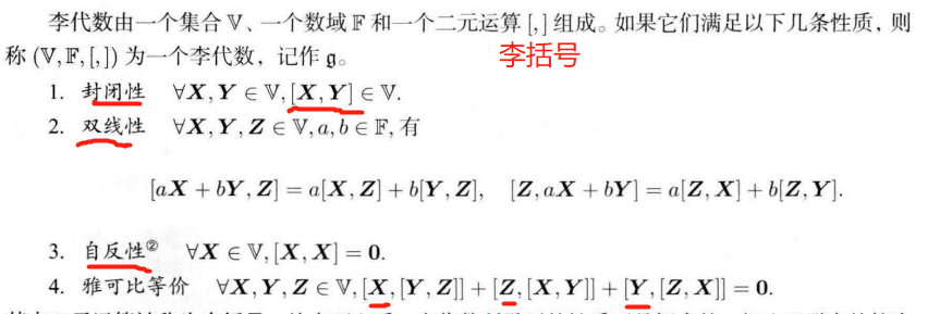
g = ( R 3 , R , × ) \mathfrak{g}=(\mathbb{R}^3, \mathbb{R}, \times) g=(R3,R,×)构成了一个李代数
4.1.4 李代数 so(3)
s o ( 3 ) \mathfrak{so}(3) so(3): 一个由三维向量组成的集合,每个向量对应一个反对称矩阵,可以用于表达旋转矩阵的导数。
s o ( 3 ) = { ϕ ∈ R 3 , Φ = ϕ ˆ ∈ R 3 × 3 } \mathfrak{so}(3)=\{\phi\in\mathbb{R}^3,\bm{\Phi}=\phi\^{}\in\mathbb{R}^{3\times3}\} so(3)={ϕ∈R3,Φ=ϕˆ∈R3×3}


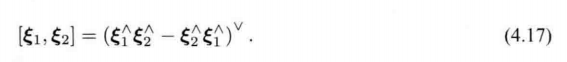
4.1.5 李代数 se(3)
李群 S E ( 3 ) SE(3) SE(3) 对应的李代数 s e ( 3 ) \mathfrak{se}(3) se(3)


4.2 指数与对数映射
4.2.1 SO(3)上的指数映射
s o ( 3 ) \mathfrak{so}(3) so(3): 旋转向量 组成的空间
指数映射: 罗德里格斯公式
R = e x p ( ϕ ∧ ) = e x p ( θ a ∧ ) = c o s θ I + ( 1 − c o s θ ) a a T + s i n θ a ∧ \bm{R}=exp(\phi^{\land})=exp(\theta\bm{a}^{\land})=cos\theta\bm{I} + (1-cos\theta)\bm{a}\bm{a}^T+sin\theta\bm{a}^{\land} R=exp(ϕ∧)=exp(θa∧)=cosθI+(1−cosθ)aaT+sinθa∧
对数映射: 李群 S O ( 3 ) SO(3) SO(3) 中的元素 ——> 李代数 s o ( 3 ) \mathfrak{so}(3) so(3)

把旋转角固定在 ± π ±\pi ±π 之间,则李群和李代数 元素 一一对应。
————————————————
罗德里格斯公式推导

e x p ( ϕ ∧ ) = e x p ( θ a ∧ ) = ∑ n = 0 ∞ 1 n ! ( θ a ∧ ) n n = 0 , 1 , 2 , 3 , . . . 原式 = I + θ a ∧ + 1 2 ! θ 2 a ∧ a ∧ + 1 3 ! θ 3 a ∧ a ∧ a ∧ + 1 4 ! θ 4 ( a ∧ ) 4 + ⋅ ⋅ ⋅ 将 a ∧ a ∧ = a a T − I ; a ∧ a ∧ a ∧ = ( a ∧ ) 3 = − a ∧ 代入 原式 = a a T − a ∧ a ∧ + θ a ∧ + 1 2 ! θ 2 a ∧ a ∧ − 1 3 ! θ 3 a ∧ − 1 4 ! θ 4 ( a ∧ ) 2 + ⋅ ⋅ ⋅ = a a T + ( θ − 1 3 ! θ 3 + 1 5 ! θ 5 − ⋅ ⋅ ⋅ ) a ∧ − ( 1 − 1 2 ! θ 2 + 1 4 ! θ 4 − ⋅ ⋅ ⋅ ) a ∧ a ∧ = a ∧ a ∧ + I + s i n θ a ∧ − c o s θ a ∧ a ∧ = ( 1 − c o s θ ) a ∧ a ∧ + I + s i n θ a ∧ = ( 1 − c o s θ ) ( a a T − I ) + I + s i n θ a ∧ = c o s θ I + ( 1 − c o s θ ) a a T + s i n θ a ∧ \begin{align*}exp(\phi^{\land}) &=exp(\theta\bm{a}^{\land})=\sum\limits_{n=0}^{\infty}\frac{1}{n!} (\theta\bm{a}^{\land})^n \\ & n = 0, 1, 2, 3, ... \\ 原式 & = \bm{I} + \theta\bm{a}^{\land} + \frac{1}{2!}\theta^2\bm{a}^{\land}\bm{a}^{\land} + \frac{1}{3!}\theta^3\bm{a}^{\land}\bm{a}^{\land}\bm{a}^{\land} +\frac{1}{4!}\theta^4(\bm{a}^{\land})^4+···\\ & 将\bm{a}^{\land}\bm{a}^{\land} = \bm{a}\bm{a}^T - \bm{I}; \bm{a}^{\land}\bm{a}^{\land}\bm{a}^{\land} = (\bm{a}^{\land})^3 =-\bm{a}^{\land} 代入 \\ 原式& = \bm{a}\bm{a}^T - \bm{a}^{\land}\bm{a}^{\land} + \theta\bm{a}^{\land} + \frac{1}{2!}\theta^2\bm{a}^{\land}\bm{a}^{\land}-\frac{1}{3!}\theta^3\bm{a}^{\land}-\frac{1}{4!}\theta^4(\bm{a}^{\land})^2+···\\ & = \bm{a}\bm{a}^T + (\theta - \frac{1}{3!}\theta^3+\frac{1}{5!}\theta^5-···)\bm{a}^{\land}-(1-\frac{1}{2!}\theta^2+\frac{1}{4!}\theta^4-···)\bm{a}^{\land}\bm{a}^{\land}\\ & = \bm{a}^{\land}\bm{a}^{\land} + \bm{I}+sin\theta \bm{a}^{\land}-cos\theta\bm{a}^{\land}\bm{a}^{\land}\\ &=(1-cos\theta)\bm{a}^{\land}\bm{a}^{\land}+\bm{I} + sin\theta\bm{a}^{\land}\\ &= (1-cos\theta)(\bm{a}\bm{a}^T-\bm{I})+\bm{I} + sin\theta\bm{a}^{\land}\\ & = cos\theta\bm{I}+ (1-cos\theta)\bm{a}\bm{a}^T + sin\theta\bm{a}^{\land} \end{align*} exp(ϕ∧)原式原式=exp(θa∧)=n=0∑∞n!1(θa∧)nn=0,1,2,3,...=I+θa∧+2!1θ2a∧a∧+3!1θ3a∧a∧a∧+4!1θ4(a∧)4+⋅⋅⋅将a∧a∧=aaT−I;a∧a∧a∧=(a∧)3=−a∧代入=aaT−a∧a∧+θa∧+2!1θ2a∧a∧−3!1θ3a∧−4!1θ4(a∧)2+⋅⋅⋅=aaT+(θ−3!1θ3+5!1θ5−⋅⋅⋅)a∧−(1−2!1θ2+4!1θ4−⋅⋅⋅)a∧a∧=a∧a∧+I+sinθa∧−cosθa∧a∧=(1−cosθ)a∧a∧+I+sinθa∧=(1−cosθ)(aaT−I)+I+sinθa∧=cosθI+(1−cosθ)aaT+sinθa∧
e x p ( θ a ∧ ) = c o s θ I + ( 1 − c o s θ ) a a T + s i n θ a ∧ exp(\theta\bm{a}^{\land})=cos\theta\bm{I} + (1-cos\theta)\bm{a}\bm{a}^T+sin\theta\bm{a}^{\land} exp(θa∧)=cosθI+(1−cosθ)aaT+sinθa∧
—————

$\bm{a}^{\land}$
a ∧ \bm{a}^{\land} a∧
————————————————
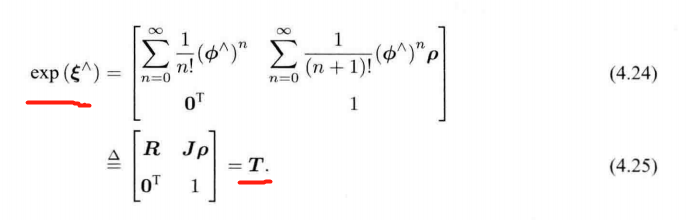
4.2.2 SE(3) 上的指数映射
——————
推导:
∑ n = 0 ∞ 1 ( n + 1 ) ! ( ϕ ∧ ) n = ∑ n = 0 ∞ 1 ( n + 1 ) ! ( θ a ∧ ) n = I + 1 2 ! θ a ∧ + 1 3 ! θ 2 ( a ∧ ) 2 + 1 4 ! θ 3 ( a ∧ ) 3 + 1 5 ! θ 4 ( a ∧ ) 4 + ⋅ ⋅ ⋅ = 1 θ ( 1 2 ! θ 2 − 1 4 ! θ 4 + ⋅ ⋅ ⋅ ) a ∧ + 1 θ ( 1 3 ! θ 3 − 1 5 ! θ 5 + ⋅ ⋅ ⋅ ) ( a ∧ ) 2 + I = 1 θ ( 1 − c o s θ ) a ∧ + 1 θ ( θ − s i n θ ) ( a a T − I ) + I = s i n θ θ I + ( 1 − s i n θ θ ) a a T + 1 − c o s θ θ a ∧ = d e f J \begin{align*} \sum\limits_{n=0}^{\infty}\frac{1}{(n+1)!}(\phi^{\land})^n &= \sum\limits_{n=0}^{\infty}\frac{1}{(n+1)!}(\theta\bm{a}^{\land})^n\\ & = \bm{I} + \frac{1}{2!}\theta\bm{a}^{\land} + \frac{1}{3!}\theta^2(\bm{a}^{\land})^2 + \frac{1}{4!}\theta^3(\bm{a}^{\land})^3 + \frac{1}{5!}\theta^4(\bm{a}^{\land})^4+···\\ & = \frac{1}{\theta}( \frac{1}{2!}\theta^2- \frac{1}{4!}\theta^4+···)\bm{a}^{\land} + \frac{1}{\theta}( \frac{1}{3!}\theta^3- \frac{1}{5!}\theta^5+···)(\bm{a}^{\land})^2+\bm{I} \\ & = \frac{1}{\theta}( 1-cos\theta)\bm{a}^{\land} + \frac{1}{\theta}(\theta-sin\theta)(\bm{a}\bm{a}^T-\bm{I})+\bm{I} \\ & = \frac{sin\theta}{\theta}\bm{I}+(1-\frac{sin\theta}{\theta})\bm{a}\bm{a}^T + \frac{1-cos\theta}{\theta}\bm{a}^{\land}\\ & \overset{\mathrm{def}}{=} \bm{J} \end{align*} n=0∑∞(n+1)!1(ϕ∧)n=n=0∑∞(n+1)!1(θa∧)n=I+2!1θa∧+3!1θ2(a∧)2+4!1θ3(a∧)3+5!1θ4(a∧)4+⋅⋅⋅=θ1(2!1θ2−4!1θ4+⋅⋅⋅)a∧+θ1(3!1θ3−5!1θ5+⋅⋅⋅)(a∧)2+I=θ1(1−cosθ)a∧+θ1(θ−sinθ)(aaT−I)+I=θsinθI+(1−θsinθ)aaT+θ1−cosθa∧=defJ
J = s i n θ θ I + ( 1 − s i n θ θ ) a a T + 1 − c o s θ θ a ∧ \bm{J}=\frac{sin\theta}{\theta}\bm{I}+(1-\frac{sin\theta}{\theta})\bm{a}\bm{a}^T + \frac{1-cos\theta}{\theta}\bm{a}^{\land} J=θsinθI+(1−θsinθ)aaT+θ1−cosθa∧
R = c o s θ I + ( 1 − c o s θ ) a a T + s i n θ a ∧ \bm{R}=cos\theta\bm{I}+(1-cos\theta)\bm{a}\bm{a}^T + sin\theta\bm{a}^{\land} R=cosθI+(1−cosθ)aaT+sinθa∧
————
t = J ρ \bm{t=Jρ} t=Jρ
平移部分发生了一次以 J \bm{J} J 为系数矩阵的 线性变换。
SO(3),SE(3),so(3),se(3)的对应关系

4.3 李代数求导与扰动模型
Baker-Campbell-Hausdorff公式(BCH公式)


4.3.2 SO(3)上的李代数求导
位姿由SO(3)上的旋转矩阵 或 SE(3)上的变换矩阵 描述
设某时刻机器人的位姿为 T \bm{T} T, 观察到了一个世界坐标位于 p \bm{p} p 的点,产生了一个观测数据 z \bm{z} z
计算理想的观测与实际数据之间的误差: e = z − T p \bm{e = z-Tp} e=z−Tp
假设一共有 N N N 个这样的路标点和观测,对机器人进行位姿估计,相当于寻找一个最优的 T \bm{T} T ,使得整体误差最小化:
min T J ( T ) = ∑ i = 1 N ∣ ∣ z i − T p i ∣ ∣ 2 2 \min\limits_{\bm{T}}J(\bm{T}) = \sum\limits_{i=1}^{N}||\bm{z_i-Tp_i}||_2^2 TminJ(T)=i=1∑N∣∣zi−Tpi∣∣22
求解上述问题,需要计算目标函数 J J J 关于变换矩阵 T \bm{T} T 的导数。
使用 李代数 解决 求导问题 的2种思路:
1、用李代数表示姿态,然后根据李代数加法对李代数求导。
2、对李群左乘或右乘微小扰动,然后对该扰动求导,称为左扰动和右扰动模型。
4.3.3 李代数求导

——————
推导:
∂ ( R p ) ∂ R = R 对应的李代数为 ϕ ∂ ( exp ( ϕ ∧ ) p ) ∂ ϕ = lim Δ ϕ → 0 exp ( ( ϕ + Δ ϕ ) ∧ ) p − exp ( ϕ ∧ ) p Δ ϕ 由式 ( 4.35 ) = lim Δ ϕ → 0 exp ( ( J l Δ ϕ ) ∧ ) exp ( ϕ ∧ ) p − exp ( ϕ ∧ ) p Δ ϕ = lim Δ ϕ → 0 ( I + ( J l Δ ϕ ) ∧ ) exp ( ϕ ∧ ) p − exp ( ϕ ∧ ) p Δ ϕ = lim Δ ϕ → 0 ( J l Δ ϕ ) ∧ exp ( ϕ ∧ ) p Δ ϕ a ∧ 等效于 a × , 因此根据叉乘的性质 = lim Δ ϕ → 0 − ( exp ( ϕ ∧ ) p ) ∧ J l Δ ϕ Δ ϕ = − ( R p ) ∧ J l \begin{align*}\frac{\partial(\bm{Rp})}{\partial\bm{R}} &\xlongequal{R对应的李代数为\phi}\frac{\partial(\exp(\phi^{\land})\bm{p})}{\partial\phi} \\ & = \lim\limits_{Δ\phi\to0}\frac{\exp((\phi+Δ\phi)^{\land})\bm{p}-\exp(\phi^{\land})\bm{p}}{Δ\phi} \\ & 由 式(4.35)\\ & = \lim\limits_{Δ\phi\to0}\frac{\exp((\bm{J}_lΔ\phi)^{\land})\exp(\phi^{\land})\bm{p}-\exp(\phi^{\land})\bm{p}}{Δ\phi} \\ & = \lim\limits_{Δ\phi\to0}\frac{(\bm{I}+(\bm{J}_lΔ\phi)^{\land})\exp(\phi^{\land})\bm{p}-\exp(\phi^{\land})\bm{p}}{Δ\phi} \\ & = \lim\limits_{Δ\phi\to0}\frac{(\bm{J}_lΔ\phi)^{\land}\exp(\phi^{\land})\bm{p}}{Δ\phi} \\ & a^{\land} 等效于 a \times ,因此根据叉乘的性质 \\ & = \lim\limits_{Δ\phi\to0}\frac{-(\exp(\phi^{\land})\bm{p})^{\land}\bm{J}_lΔ\phi}{Δ\phi} \\ & = -(\bm{Rp})^{\land}\bm{J}_l \end{align*} ∂R∂(Rp)R对应的李代数为ϕ∂ϕ∂(exp(ϕ∧)p)=Δϕ→0limΔϕexp((ϕ+Δϕ)∧)p−exp(ϕ∧)p由式(4.35)=Δϕ→0limΔϕexp((JlΔϕ)∧)exp(ϕ∧)p−exp(ϕ∧)p=Δϕ→0limΔϕ(I+(JlΔϕ)∧)exp(ϕ∧)p−exp(ϕ∧)p=Δϕ→0limΔϕ(JlΔϕ)∧exp(ϕ∧)pa∧等效于a×,因此根据叉乘的性质=Δϕ→0limΔϕ−(exp(ϕ∧)p)∧JlΔϕ=−(Rp)∧Jl
∂ ( exp ( ϕ ∧ ) p ) ∂ ϕ = − ( R p ) ∧ J l \frac{\partial(\exp(\phi^{\land})\bm{p})}{\partial\phi} = -(\bm{Rp})^{\land}\bm{J}_l ∂ϕ∂(exp(ϕ∧)p)=−(Rp)∧Jl
——————
4.3.4 扰动模型(左乘)【更简单 的导数计算模型】
对 R \bm{R} R 进行一次扰动 Δ R Δ\bm{R} ΔR ,看结果对于 扰动的变化率。
设左扰动 Δ R Δ\bm{R} ΔR 对应的李代数 为 φ \varphi φ
∂ ( R p ) ∂ φ = lim φ → 0 exp ( φ ∧ ) exp ( ϕ ∧ ) p − exp ( ϕ ∧ ) p φ = lim φ → 0 ( I + φ ∧ ) exp ( ϕ ∧ ) p − exp ( ϕ ∧ ) p φ = lim φ → 0 φ ∧ exp ( ϕ ∧ ) p φ = lim φ → 0 φ ∧ R p φ = lim φ → 0 − ( R p ) ∧ φ φ = − ( R p ) ∧ \begin{align*}\frac{\partial(\bm{Rp})}{\partial\varphi} &= \lim\limits_{\varphi\to0}\frac{\exp(\varphi^{\land})\exp(\phi^{\land})\bm{p}-\exp(\phi^{\land})\bm{p}}{\varphi}\\ &= \lim\limits_{\varphi\to0}\frac{(\bm{I} + \varphi^{\land})\exp(\phi^{\land})\bm{p}-\exp(\phi^{\land})\bm{p}}{\varphi}\\ &= \lim\limits_{\varphi\to0}\frac{\varphi^{\land}\exp(\phi^{\land})\bm{p}}{\varphi}\\ &= \lim\limits_{\varphi\to0}\frac{\varphi^{\land}\bm{Rp}}{\varphi}\\ &= \lim\limits_{\varphi\to0}\frac{-(\bm{Rp})^{\land}\varphi}{\varphi}\\ &= -(\bm{Rp})^{\land} \end{align*} ∂φ∂(Rp)=φ→0limφexp(φ∧)exp(ϕ∧)p−exp(ϕ∧)p=φ→0limφ(I+φ∧)exp(ϕ∧)p−exp(ϕ∧)p=φ→0limφφ∧exp(ϕ∧)p=φ→0limφφ∧Rp=φ→0limφ−(Rp)∧φ=−(Rp)∧
4.3.5 SE(3)上的李代数求导
假设某空间点 p \bm{p} p 经过一次变换 T \bm{T} T (对应李代数为 ξ \bm{\xi} ξ), 得到 T p \bm{Tp} Tp
现在给 T \bm{T} T 左乘一个扰动 Δ T = exp ( Δ ξ ∧ ) Δ\bm{T} = \exp(Δ\bm{\xi}^{\land}) ΔT=exp(Δξ∧)
设扰动项的李代数为 Δ ξ = [ Δ ρ , Δ ϕ ] T Δ\bm{\xi}=[Δ\bm{\rho},Δ\bm{\phi}]^T Δξ=[Δρ,Δϕ]T,则

∂ ( T p ) ∂ Δ ξ = lim Δ ξ → 0 exp ( Δ ξ ∧ ) exp ( ξ ∧ ) p − exp ( ξ ∧ ) p Δ ξ = lim Δ ξ → 0 ( I + Δ ξ ∧ ) exp ( ξ ∧ ) p − exp ( ξ ∧ ) p Δ ξ = lim Δ ξ → 0 Δ ξ ∧ exp ( ξ ∧ ) p Δ ξ = lim Δ ξ → 0 [ Δ ϕ ∧ Δ ρ 0 T 0 ] [ R p + t 1 ] Δ ξ = lim Δ ξ → 0 [ Δ ϕ ∧ ( R p + t ) + Δ ρ 0 T ] [ Δ ρ , Δ ϕ ] T = [ I − ( R p + t ) ∧ 0 T 0 T ] = d e f ( T p ) ⨀ \begin{align*}\frac{\partial(\bm{Tp})}{\partial{Δ\bm{\xi}}} &= \lim\limits_{Δ\bm{\xi}\to0}\frac{\exp(Δ\bm{\xi}^{\land})\exp(\bm{\xi}^{\land})\bm{p}-\exp(\bm{\xi}^{\land})\bm{p}}{Δ\bm{\xi}} \\ &= \lim\limits_{Δ\bm{\xi}\to0}\frac{(\bm{I} +Δ\bm{\xi}^{\land})\exp(\bm{\xi}^{\land})\bm{p}-\exp(\bm{\xi}^{\land})\bm{p}}{Δ\bm{\xi}} \\ &= \lim\limits_{Δ\bm{\xi}\to0}\frac{Δ\bm{\xi}^{\land}\exp(\bm{\xi}^{\land})\bm{p}}{Δ\bm{\xi}} \\ &=\lim\limits_{Δ\bm{\xi}\to0} \frac{\begin{bmatrix} Δ\bm{\phi}^{\land} & \Delta\bm{\rho}\\ \bm{0}^T & 0 \end{bmatrix}\begin{bmatrix} \bm{Rp+t}\\ 1 \end{bmatrix}}{Δ\bm{\xi}}\\ &=\lim\limits_{Δ\bm{\xi}\to0} \frac{\begin{bmatrix} \Delta\bm{\phi}^{\land}(\bm{Rp+t})+\Delta\bm{\rho}\\ \bm{0}^T \end{bmatrix}}{[Δ\bm{\rho},Δ\bm{\phi}]^T} \\ & = \begin{bmatrix} \bm{I} & -(\bm{Rp+t})^{\land} \\ \bm{0}^T & \bm{0}^T \end{bmatrix} \\ &\overset{\mathrm{def}}{=}(\bm{Tp})^{\bigodot} \end{align*} ∂Δξ∂(Tp)=Δξ→0limΔξexp(Δξ∧)exp(ξ∧)p−exp(ξ∧)p=Δξ→0limΔξ(I+Δξ∧)exp(ξ∧)p−exp(ξ∧)p=Δξ→0limΔξΔξ∧exp(ξ∧)p=Δξ→0limΔξ[Δϕ∧0TΔρ0][Rp+t1]=Δξ→0lim[Δρ,Δϕ]T[Δϕ∧(Rp+t)+Δρ0T]=[I0T−(Rp+t)∧0T]=def(Tp)⨀

$\overset{\mathrm{def}}{=}(\bm{Tp})^{\bigodot}$
4.4 Sophus应用 【Code】
SO(3)、SE(3)
二维运动SO(2)和SE(2)
相似变换 Sim(3)
mkdir build && cd build
cmake ..
make
./useSophus
CMakeLists.txt
cmake_minimum_required(VERSION 2.8)project(useSophus)find_package(Sophus REQUIRED)
include_directories( ${Sophus_INCLUDE_DIRS})add_executable(useSophus useSophus.cpp)
target_link_libraries(useSophus ${Sophus_LIBRARIES})
#include<iostream>
#include<cmath>
#include<Eigen/Core>
#include<Eigen/Geometry>
#include "sophus/se3.h"using namespace std;
using namespace Eigen;/* sophus 的基本用法 */
int main(int argc, char **argv){// 沿 Z轴  转90° 的旋转矩阵Matrix3d R = AngleAxisd(M_PI/2, Vector3d(0, 0, 1)).toRotationMatrix();/* 四元数 */Quaterniond q(R);Sophus::SO3 SO3_R(R);Sophus::SO3 SO3_q(q);cout << "SO(3) from matrix:\n" << SO3_R.matrix() << endl;cout << "SO(3) from quatenion:\n" << SO3_q.matrix() << endl;cout << "they are equal" << endl;return 0;
}

#include<iostream>
#include<cmath>
#include<Eigen/Core>
#include<Eigen/Geometry>
#include "sophus/se3.h"using namespace std;
using namespace Eigen;/* sophus 的基本用法 */
int main(int argc, char **argv){/* 使用 对数映射 获得  李代数*/Matrix3d R = AngleAxisd(M_PI/2, Vector3d(0, 0, 1)).toRotationMatrix();Sophus::SO3 SO3_R(R);Vector3d so3 = SO3_R.log();cout << "so3 = " << so3.transpose() << endl;// hat  向量 ——> 反对称矩阵cout << "so3 hat = \n" << Sophus::SO3::hat(so3)<< endl;// vee  反对称 ——> 向量cout << "so3 hat vee = " << Sophus::SO3::vee(Sophus::SO3::hat(so3)).transpose() << endl;Vector3d update_so3(1e-4, 0, 0);// 假设更新量为这么多Sophus::SO3 SO3_updated =Sophus::SO3::exp(update_so3) * SO3_R;cout << "SO3 updated = \n" << SO3_updated.matrix() << endl;return 0;
}

#include<iostream>
#include<cmath>
#include<Eigen/Core>
#include<Eigen/Geometry>
#include "sophus/se3.h"using namespace std;
using namespace Eigen;/* sophus   SE(3) 的基本用法 */
int main(int argc, char **argv){Matrix3d R = AngleAxisd(M_PI/2, Vector3d(0, 0, 1)).toRotationMatrix();  // 沿 Z轴 旋转 90° 的旋转矩阵Vector3d t(1, 0, 0);  // 沿 X 轴平移1Sophus::SE3 SE3_Rt(R, t);  // 从R,t 构造 SE(3)Quaterniond q(R);Sophus::SE3 SE3_qt(q, t); // 从q, t 构造 SE(3)cout << "SE3 from R, t = \n" << SE3_Rt.matrix() << endl;cout << "SE3 from q, t = \n" << SE3_qt.matrix() << endl; /* 李代数se(3) 是一个 6 维 向量*/typedef Eigen::Matrix<double, 6, 1> Vector6d;Vector6d se3 = SE3_Rt.log();cout << "se3 = " << se3.transpose() << endl;// hat  向量 ——> 反对称矩阵cout << "se3 hat = \n" << Sophus::SE3::hat(se3)<< endl;// vee  反对称 ——> 向量cout << "se3 hat vee = " << Sophus::SE3::vee(Sophus::SE3::hat(se3)).transpose() << endl;// 更新Vector6d update_se3;// 更新量update_se3.setZero();update_se3(0, 0) = 1e-4;Sophus::SE3 SE3_updated =Sophus::SE3::exp(update_se3) * SE3_Rt;cout << "SE3 updated = \n" << SE3_updated.matrix() << endl;return 0;
}

4.4.2 评估轨迹的误差 【Code】
————————
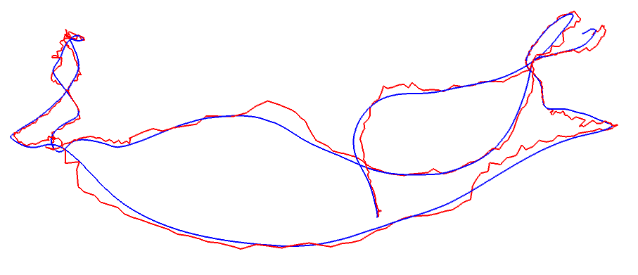
考虑一条估计轨迹 T e s t i , i \bm{T}_{esti,i} Testi,i 和真实轨迹 T g t , i \bm{T}_{gt,i} Tgt,i ,其中 i = 1 , ⋅ ⋅ ⋅ , N i= 1,···,N i=1,⋅⋅⋅,N
1、绝对误差轨迹(Absolute Trajectory Error, ATE) 旋转和平移误差
A T E a l l = 1 N ∑ i = 1 N ∣ ∣ l o g ( T g t , i − 1 T e s t i , i ) ∨ ∣ ∣ 2 2 ATE_{all}=\sqrt{\frac{1}{N}\sum\limits_{i=1}^{N}||log(\bm{T}_{gt,i}^{-1}\bm{T}_{esti,i})^{\vee}||_2^2} ATEall=N1i=1∑N∣∣log(Tgt,i−1Testi,i)∨∣∣22
- 每个位姿 李代数 的均方根误差 (Root-Mean-Squared Error,RMSE)
2、绝对平移误差(Average Translational Error)
A T E t r a n s = 1 N ∑ i = 1 N ∣ ∣ t r a n s ( T g t , i − 1 T e s t i , i ) ∣ ∣ 2 2 ATE_{trans}=\sqrt{\frac{1}{N}\sum\limits_{i=1}^{N}||trans(\bm{T}_{gt,i}^{-1}\bm{T}_{esti,i})||_2^2} ATEtrans=N1i=1∑N∣∣trans(Tgt,i−1Testi,i)∣∣22
其中 trans 表示 取括号内部变量的平移部分。
- 从整条轨迹上看,旋转出现偏差后,随后的轨迹在平移上也会出现误差。
3、相对误差
考虑 i i i 时刻到 i + Δ t i+\Delta t i+Δt 的运动,相对位姿误差(Relative Pose Error, RPE)
R P E a l l = 1 N − Δ t ∑ i = 1 N − Δ t ∣ ∣ l o g ( ( T g t , i − 1 T g t , i + Δ t ) − 1 ( T e s t i , i − 1 T e s t i , i + Δ t ) ) ∨ ∣ ∣ 2 2 RPE_{all}=\sqrt{\frac{1}{N-\Delta t}\sum\limits_{i=1}^{N-\Delta t}||log((\bm{T}_{gt,i}^{-1}\bm{T}_{gt,i+\Delta t})^{-1}(\bm{T}_{esti,i}^{-1}\bm{T}_{esti,i+\Delta t}))^{\vee}||_2^2} RPEall=N−Δt1i=1∑N−Δt∣∣log((Tgt,i−1Tgt,i+Δt)−1(Testi,i−1Testi,i+Δt))∨∣∣22
R P E t r a n s = 1 N − Δ t ∑ i = 1 N − Δ t ∣ ∣ t r a n s ( ( T g t , i − 1 T g t , i + Δ t ) − 1 ( T e s t i , i − 1 T e s t i , i + Δ t ) ) ∣ ∣ 2 2 RPE_{trans}=\sqrt{\frac{1}{N-\Delta t}\sum\limits_{i=1}^{N-\Delta t}||trans((\bm{T}_{gt,i}^{-1}\bm{T}_{gt,i+\Delta t})^{-1}(\bm{T}_{esti,i}^{-1}\bm{T}_{esti,i+\Delta t}))||_2^2} RPEtrans=N−Δt1i=1∑N−Δt∣∣trans((Tgt,i−1Tgt,i+Δt)−1(Testi,i−1Testi,i+Δt))∣∣22
————————

mkdir build && cd build
cmake ..
make
./trajectoryError
CMakeLists.txt
cmake_minimum_required(VERSION 2.8)project(trajectoryError)find_package(Sophus REQUIRED)
include_directories( ${Sophus_INCLUDE_DIRS})option(USE_UBUNTU_20 "Set to ON if you are using Ubuntu 20.04" OFF)
find_package(Pangolin REQUIRED)
if(USE_UBUNTU_20)message("You are using Ubuntu 20.04, fmt::fmt will be linked")find_package(fmt REQUIRED)set(FMT_LIBRARIES fmt::fmt)
endif()
include_directories(${Pangolin_INCLUDE_DIRS})add_executable(trajectoryError trajectoryError.cpp)
target_link_libraries(trajectoryError ${Sophus_LIBRARIES})
target_link_libraries(trajectoryError ${Pangolin_LIBRARIES} ${FMT_LIBRARIES})
trajectoryError.cpp
#include <iostream>
#include <fstream>
#include <unistd.h>
#include <pangolin/pangolin.h>
#include <sophus/se3.h>using namespace Sophus;
using namespace std;string groundtruth_file = "../groundtruth.txt";
string estimated_file = "../estimated.txt";typedef vector<Sophus::SE3, Eigen::aligned_allocator<Sophus::SE3>> TrajectoryType;void DrawTrajectory(const TrajectoryType >, const TrajectoryType &esti);TrajectoryType ReadTrajectory(const string &path);int main(int argc, char **argv) {TrajectoryType groundtruth = ReadTrajectory(groundtruth_file);TrajectoryType estimated = ReadTrajectory(estimated_file);assert(!groundtruth.empty() && !estimated.empty());assert(groundtruth.size() == estimated.size());// compute rmsedouble rmse = 0;for (size_t i = 0; i < estimated.size(); i++) {Sophus::SE3 p1 = estimated[i], p2 = groundtruth[i];double error = (p2.inverse() * p1).log().norm();rmse += error * error;}rmse = rmse / double(estimated.size());rmse = sqrt(rmse);cout << "RMSE = " << rmse << endl;DrawTrajectory(groundtruth, estimated);return 0;
}TrajectoryType ReadTrajectory(const string &path) {ifstream fin(path);TrajectoryType trajectory;if (!fin) {cerr << "trajectory " << path << " not found." << endl;return trajectory;}while (!fin.eof()) {double time, tx, ty, tz, qx, qy, qz, qw;fin >> time >> tx >> ty >> tz >> qx >> qy >> qz >> qw;Sophus::SE3 p1(Eigen::Quaterniond(qw, qx, qy, qz), Eigen::Vector3d(tx, ty, tz));trajectory.push_back(p1);}return trajectory;
}void DrawTrajectory(const TrajectoryType >, const TrajectoryType &esti) {// create pangolin window and plot the trajectorypangolin::CreateWindowAndBind("Trajectory Viewer", 1024, 768);glEnable(GL_DEPTH_TEST);glEnable(GL_BLEND);glBlendFunc(GL_SRC_ALPHA, GL_ONE_MINUS_SRC_ALPHA);pangolin::OpenGlRenderState s_cam(pangolin::ProjectionMatrix(1024, 768, 500, 500, 512, 389, 0.1, 1000),pangolin::ModelViewLookAt(0, -0.1, -1.8, 0, 0, 0, 0.0, -1.0, 0.0));pangolin::View &d_cam = pangolin::CreateDisplay().SetBounds(0.0, 1.0, pangolin::Attach::Pix(175), 1.0, -1024.0f / 768.0f).SetHandler(new pangolin::Handler3D(s_cam));while (pangolin::ShouldQuit() == false) {glClear(GL_COLOR_BUFFER_BIT | GL_DEPTH_BUFFER_BIT);d_cam.Activate(s_cam);glClearColor(1.0f, 1.0f, 1.0f, 1.0f);glLineWidth(2);for (size_t i = 0; i < gt.size() - 1; i++) {glColor3f(0.0f, 0.0f, 1.0f); // blue for ground truthglBegin(GL_LINES);auto p1 = gt[i], p2 = gt[i + 1];glVertex3d(p1.translation()[0], p1.translation()[1], p1.translation()[2]);glVertex3d(p2.translation()[0], p2.translation()[1], p2.translation()[2]);glEnd();}for (size_t i = 0; i < esti.size() - 1; i++) {glColor3f(1.0f, 0.0f, 0.0f); // red for estimatedglBegin(GL_LINES);auto p1 = esti[i], p2 = esti[i + 1];glVertex3d(p1.translation()[0], p1.translation()[1], p1.translation()[2]);glVertex3d(p2.translation()[0], p2.translation()[1], p2.translation()[2]);glEnd();}pangolin::FinishFrame();usleep(5000); // sleep 5 ms}}
4.5 相似变换群 与 李代数
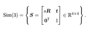
单目视觉 相似变换群Sim(3)
尺度不确定性 与 尺度漂移
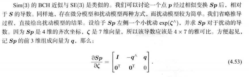
对位于空间的点 p \bm{p} p ,在相机坐标系下要经过一个相似变换。
p ′ = [ s R t 0 T 1 ] p = s R p + t \bm{p}^{\prime}=\begin{bmatrix}s\bm{R} & \bm{t}\\ \bm{0}^T& 1 \end{bmatrix}\bm{p} = s\bm{Rp+t} p′=[sR0Tt1]p=sRp+t


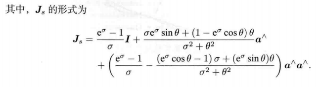

对于尺度因子,李群中的 s s s 即为李代数中 σ \sigma σ 的指数函数
4.6 小结
李群 SO(3) 和 SE(3) 以及对应的李代数 s o ( 3 ) \mathfrak{so}(3) so(3) 和 s e ( 3 ) \mathfrak{se}(3) se(3)
BCH 线性近似, 对位姿进行扰动并求导
习题


题1
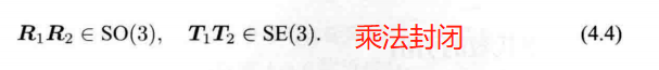
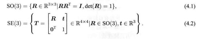
验证SO(3)、SE(3)、Sim(3)关于乘法成群
特殊正交群SO(n) 旋转矩阵群
特殊欧式群SE(n) n维欧式变换


题2

题4

√ 题5

证明:
原式等效于证明 R p ∧ R T R = ( R p ) ∧ R R p ∧ I = ( R p ) ∧ R R p ∧ = ( R p ) ∧ R 对于向量 v ∈ R 3 R p ∧ v = ( R p ) ∧ R v 上式等号左边 表示向量 p , v 叉乘后所得向量根据 R 旋转。 等号右边表示 向量 p , v 分别根据 R 旋转后叉乘,显然得到同一个向量。 证毕。 \begin{align*} 原式等效于证明\\ \bm{Rp^{\land}R^TR} & = \bm{(Rp)}^{\land}\bm{R} \\ \bm{Rp^{\land}\bm{I}} & = \bm{(Rp)}^{\land}\bm{R} \\ \bm{Rp^{\land}} & = \bm{(Rp)}^{\land}\bm{R} \\ 对于向量 \bm{v} \in \mathbb{R}^3\\ \bm{Rp^{\land}}\bm{v} & = \bm{(Rp)}^{\land}\bm{R}\bm{v} \\ 上式等号左边& 表示向量\bm{p,v}叉乘后所得向量根据 \bm{R}旋转。\\ 等号右边表示& 向量\bm{p,v}分别根据 \bm{R}旋转后叉乘,显然得到同一个向量。\\ 证毕。 \end{align*} 原式等效于证明Rp∧RTRRp∧IRp∧对于向量v∈R3Rp∧v上式等号左边等号右边表示证毕。=(Rp)∧R=(Rp)∧R=(Rp)∧R=(Rp)∧Rv表示向量p,v叉乘后所得向量根据R旋转。向量p,v分别根据R旋转后叉乘,显然得到同一个向量。
√ 题6
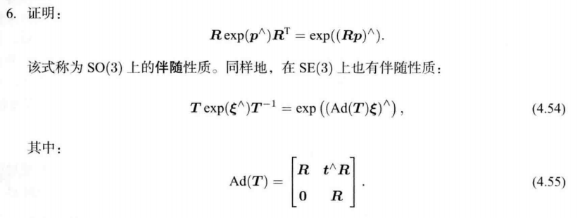
根据题 5 的结论 : ( R p ) ∧ = R p ∧ R T exp ( ( R p ) ∧ ) = exp ( R p ∧ R T ) 级数展开 = ∑ n = 0 ∞ ( R p ∧ R T ) n N ! = ∑ n = 0 ∞ R p ∧ R T ⋅ R p ∧ R T ⋅ , ⋅ ⋅ ⋅ , ⋅ R p ∧ R T ⋅ R p ∧ R T N ! 其中 R T R = I = ∑ n = 0 ∞ R ( p ∧ ) n R T N ! = R ∑ n = 0 ∞ ( p ∧ ) n N ! R T = R exp ( p ∧ ) R T \begin{align*}根据题5 的结论&:\bm{(Rp)}^{\land} = \bm{Rp^{\land}R^T} \\ \exp((\bm{Rp})^{\land})& = \exp(\bm{Rp^{\land}R^T}) \\ 级数展开\\ &= \sum\limits_{n=0}^{\infty}\frac{(\bm{Rp^{\land}R^T}) ^n}{N!} \\ &= \sum\limits_{n=0}^{\infty}\frac{\bm{Rp^{\land}R^T}·\bm{Rp^{\land}R^T}·,···,·\bm{Rp^{\land}R^T}·\bm{Rp^{\land}R^T}}{N!} \\ 其中 \bm{R^TR=I}\\ & = \sum\limits_{n=0}^{\infty}\frac{\bm{R(p^{\land})^nR^T}}{{N!} }\\ & = \bm{R} \sum\limits_{n=0}^{\infty}\frac{\bm{(p^{\land})^n}}{{N!} } \bm{R}^T \\ & = \bm{R}\exp(\bm{p}^{\land})\bm{R}^T \end{align*} 根据题5的结论exp((Rp)∧)级数展开其中RTR=I:(Rp)∧=Rp∧RT=exp(Rp∧RT)=n=0∑∞N!(Rp∧RT)n=n=0∑∞N!Rp∧RT⋅Rp∧RT⋅,⋅⋅⋅,⋅Rp∧RT⋅Rp∧RT=n=0∑∞N!R(p∧)nRT=Rn=0∑∞N!(p∧)nRT=Rexp(p∧)RT
证毕。
——————
6.2 SE(3)伴随性质
T exp ( ξ ∧ ) T − 1 = T ∑ n = 0 ∞ ( ξ ∧ ) n n ! T − 1 由于 T − 1 T = I = ∑ n = 0 ∞ T ξ ∧ T − 1 ⋅ T ξ ∧ T − 1 ⋅ T ξ ∧ T − 1 ⋅ T ξ ∧ T − 1 ⋅ , ⋅ ⋅ ⋅ , T ξ ∧ T − 1 ⋅ T ξ ∧ T − 1 n ! = ∑ n = 0 ∞ ( T ξ ∧ T − 1 ) n n ! = exp ( T ξ ∧ T − 1 ) \begin{align*} \bm{T}\exp(\bm{\xi}^{\land})\bm{T}^{-1} &= \bm{T}\sum\limits_{n=0}^{\infty}\frac{(\bm{\xi}^{\land})^n}{n!}\bm{T}^{-1} \\ 由于 \bm{T^{-1}T=I} \\ & = \sum\limits_{n=0}^{\infty}\frac{\bm{T}\bm{\xi}^{\land}\bm{T}^{-1}·\bm{T}\bm{\xi}^{\land}\bm{T}^{-1}·\bm{T}\bm{\xi}^{\land}\bm{T}^{-1}·\bm{T}\bm{\xi}^{\land}\bm{T}^{-1}·,···, \bm{T}\bm{\xi}^{\land}\bm{T}^{-1}·\bm{T}\bm{\xi}^{\land}\bm{T}^{-1}}{n!} \\ & = \sum\limits_{n=0}^{\infty}\frac{(\bm{T}\bm{\xi}^{\land}\bm{T}^{-1})^n}{n!} \\ &= \exp(\bm{T}\bm{\xi}^{\land}\bm{T}^{-1}) \\ \end{align*} Texp(ξ∧)T−1由于T−1T=I=Tn=0∑∞n!(ξ∧)nT−1=n=0∑∞n!Tξ∧T−1⋅Tξ∧T−1⋅Tξ∧T−1⋅Tξ∧T−1⋅,⋅⋅⋅,Tξ∧T−1⋅Tξ∧T−1=n=0∑∞n!(Tξ∧T−1)n=exp(Tξ∧T−1)
ξ = [ ρ ϕ ] , ξ ∧ = [ ϕ ∧ ρ 0 T 0 ] , T = [ R t 0 T 1 ] , T − 1 = [ R T − R T t 0 T 1 ] \bm{\xi=}\begin{bmatrix}\bm{\rho}\\ \bm{\phi} \end{bmatrix},\bm{\xi}^{\land}=\begin{bmatrix}\bm{\phi}^{\land} & \bm{\rho} \\ \bm{0}^T & 0 \end{bmatrix},\bm{T}=\begin{bmatrix}\bm{R} & \bm{t}\\ \bm{0}^T & 1 \end{bmatrix},\bm{T}^{-1}=\begin{bmatrix}\bm{R}^T & -\bm{R}^T\bm{t}\\ \bm{0}^T & 1 \end{bmatrix} ξ=[ρϕ],ξ∧=[ϕ∧0Tρ0],T=[R0Tt1],T−1=[RT0T−RTt1]

则:
T ξ ∧ T − 1 = [ R t 0 T 1 ] [ ϕ ∧ ρ 0 T 0 ] [ R T − R T t 0 T 1 ] = [ R ϕ ∧ R ρ 0 T 0 ] [ R T − R T t 0 T 1 ] = [ R ϕ ∧ R T − R ϕ ∧ R T t + R ρ 0 T 0 ] 由题 5 的结论 R p ∧ R T = ( R p ) ∧ = [ ( R ϕ ) ∧ − ( R ϕ ) ∧ t + R ρ 0 T 0 ] 对比 ξ , ξ ∧ 进行转换 = [ − ( R ϕ ) ∧ t + R ρ R ϕ ] ∧ 由叉乘性质, = [ t ∧ R ϕ + R ρ R ϕ ] ∧ = [ R t ∧ R 0 R ] [ ρ ϕ ] ) ∧ = ( A d ( T ) ξ ) ∧ \begin{align*}\bm{T}\bm{\xi}^{\land}\bm{T}^{-1}&= \begin{bmatrix}\bm{R} & \bm{t}\\ \bm{0}^T & 1 \end{bmatrix}\begin{bmatrix}\bm{\phi}^{\land} & \bm{\rho} \\ \bm{0}^T & 0 \end{bmatrix}\begin{bmatrix}\bm{R}^T & -\bm{R}^T\bm{t}\\ \bm{0}^T & 1 \end{bmatrix}\\ &= \begin{bmatrix}\bm{R}\bm{\phi}^{\land} & \bm{R\rho}\\ \bm{0}^T & 0 \end{bmatrix}\begin{bmatrix}\bm{R}^T & -\bm{R}^T\bm{t}\\ \bm{0}^T & 1 \end{bmatrix}\\ &= \begin{bmatrix}\bm{R}\bm{\phi}^{\land}\bm{R}^T & -\bm{R}\bm{\phi}^{\land}\bm{R}^T\bm{t + \bm{R\rho}}\\ \bm{0}^T & 0 \end{bmatrix} \\ 由题5的结论& \bm{Rp^{\land}R^T} = \bm{(Rp)}^{\land} \\ &= \begin{bmatrix}(\bm{R}\bm{\phi})^{\land} & -(\bm{R}\bm{\phi})^{\land}\bm{t + \bm{R\rho}}\\ \bm{0}^T &0 \end{bmatrix}\\ & 对比 \bm{\xi, {\xi}^{\land}}进行转换\\ &= \begin{bmatrix}-(\bm{R}\bm{\phi})^{\land}\bm{t + \bm{R\rho}}\\ \bm{R}\bm{\phi} \end{bmatrix}^{\land}\\ 由叉乘性质, \\ &= \begin{bmatrix}\bm{t}^{\land}\bm{R}\bm{\phi}+ \bm{R\rho}\\ \bm{R}\bm{\phi} \end{bmatrix}^{\land}\\ &= \begin{bmatrix}\bm{R}& \bm{t}^{\land}\bm{R} \\ \bm{0} & \bm{R} \end{bmatrix}\begin{bmatrix}\bm{\rho}\\ \bm{\phi} \end{bmatrix})^{\land}\\ & = (Ad(\bm{T})\bm{\xi})^{\land} \end{align*} Tξ∧T−1由题5的结论由叉乘性质,=[R0Tt1][ϕ∧0Tρ0][RT0T−RTt1]=[Rϕ∧0TRρ0][RT0T−RTt1]=[Rϕ∧RT0T−Rϕ∧RTt+Rρ0]Rp∧RT=(Rp)∧=[(Rϕ)∧0T−(Rϕ)∧t+Rρ0]对比ξ,ξ∧进行转换=[−(Rϕ)∧t+RρRϕ]∧=[t∧Rϕ+RρRϕ]∧=[R0t∧RR][ρϕ])∧=(Ad(T)ξ)∧
综上:
T exp ( ξ ∧ ) T − 1 = exp ( ( A d ( T ) ξ ) ∧ ) \bm{T}\exp(\bm{\xi}^{\land})\bm{T}^{-1}=\exp((Ad(\bm{T})\bm{\xi})^{\land}) Texp(ξ∧)T−1=exp((Ad(T)ξ)∧)
其中
A d ( T ) = [ R t ∧ R 0 R ] Ad(\bm{T})=\begin{bmatrix}\bm{R}& \bm{t}^{\land}\bm{R} \\ \bm{0} & \bm{R} \end{bmatrix} Ad(T)=[R0t∧RR]
证毕
————————————————
√ 题7


SO(3):
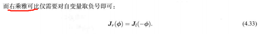
设右扰动 Δ R Δ\bm{R} ΔR 对应的李代数 为 φ \varphi φ
∂ ( R p ) ∂ φ = lim φ → 0 exp ( ϕ ∧ ) exp ( φ ∧ ) p − exp ( ϕ ∧ ) p φ = lim φ → 0 exp ( ϕ ∧ ) ( I + φ ∧ ) p − exp ( ϕ ∧ ) p φ = lim φ → 0 exp ( ϕ ∧ ) φ ∧ p φ = lim φ → 0 R φ ∧ p φ 由题 5 : R p ∧ = ( R p ) ∧ R = lim φ → 0 ( R φ ) ∧ R p φ 由叉乘性质 = lim φ → 0 − ( R p ) ∧ R φ φ = − ( R p ) ∧ R \begin{align*}\frac{\partial(\bm{Rp})}{\partial\varphi} &= \lim\limits_{\varphi\to0}\frac{\exp(\phi^{\land})\exp(\varphi^{\land})\bm{p}-\exp(\phi^{\land})\bm{p}}{\varphi}\\ &= \lim\limits_{\varphi\to0}\frac{\exp(\phi^{\land})(\bm{I} + \varphi^{\land})\bm{p}-\exp(\phi^{\land})\bm{p}}{\varphi}\\ &= \lim\limits_{\varphi\to0}\frac{\exp(\phi^{\land})\varphi^{\land}\bm{p}}{\varphi}\\ &= \lim\limits_{\varphi\to0}\frac{\bm{R}\varphi^{\land}\bm{p}}{\varphi}\\ 由题5 : \bm{Rp^{\land}} & = \bm{(Rp)}^{\land}\bm{R} \\ &= \lim\limits_{\varphi\to0}\frac{(\bm{R}\varphi)^{\land}\bm{Rp}}{\varphi}\\ 由叉乘性质\\ &= \lim\limits_{\varphi\to0}\frac{-(\bm{Rp})^{\land}\bm{R}\varphi}{\varphi}\\ & = -(\bm{Rp})^{\land}\bm{R} \end{align*} ∂φ∂(Rp)由题5:Rp∧由叉乘性质=φ→0limφexp(ϕ∧)exp(φ∧)p−exp(ϕ∧)p=φ→0limφexp(ϕ∧)(I+φ∧)p−exp(ϕ∧)p=φ→0limφexp(ϕ∧)φ∧p=φ→0limφRφ∧p=(Rp)∧R=φ→0limφ(Rφ)∧Rp=φ→0limφ−(Rp)∧Rφ=−(Rp)∧R
SE(3):
假设某空间点 p \bm{p} p 经过一次变换 T \bm{T} T (对应李代数为 ξ \bm{\xi} ξ), 得到 T p \bm{Tp} Tp
现在给 T \bm{T} T 右乘一个扰动 Δ T = exp ( Δ ξ ∧ ) Δ\bm{T} = \exp(Δ\bm{\xi}^{\land}) ΔT=exp(Δξ∧)
设扰动项的李代数为 Δ ξ = [ Δ ρ , Δ ϕ ] T Δ\bm{\xi}=[Δ\bm{\rho},Δ\bm{\phi}]^T Δξ=[Δρ,Δϕ]T,则
∂ ( T p ) ∂ Δ ξ = lim Δ ξ → 0 exp ( ξ ∧ ) exp ( Δ ξ ∧ ) p − exp ( ξ ∧ ) p Δ ξ = lim Δ ξ → 0 exp ( ξ ∧ ) ( I + Δ ξ ∧ ) p − exp ( ξ ∧ ) p Δ ξ = lim Δ ξ → 0 exp ( ξ ∧ ) Δ ξ ∧ p Δ ξ = lim Δ ξ → 0 [ R t 0 1 ] [ Δ ϕ ∧ Δ ρ 0 T 0 ] p Δ ξ 把 p 前的 矩阵当做旋转矩阵,结合向量旋转的性质, = lim Δ ξ → 0 [ R t 0 1 ] [ Δ ϕ ∧ p + Δ ρ 0 ] Δ ξ = lim Δ ξ → 0 [ R Δ ϕ ∧ p + R Δ ρ 0 T ] [ Δ ρ , Δ ϕ ] T 将 Δ ρ , Δ ϕ 提出来,方便求导 根据 R p ∧ = ( R p ) ∧ R = lim Δ ξ → 0 [ ( R Δ ϕ ) ∧ R p + R Δ ρ 0 T ] [ Δ ρ , Δ ϕ ] T = lim Δ ξ → 0 [ − ( R p ) ∧ R Δ ϕ + R Δ ρ 0 T ] [ Δ ρ , Δ ϕ ] T = [ R − ( R p ) ∧ R 0 T 0 T ] \begin{align*}\frac{\partial(\bm{Tp})}{\partial{Δ\bm{\xi}}} &= \lim\limits_{Δ\bm{\xi}\to0}\frac{\exp(\bm{\xi}^{\land})\exp(Δ\bm{\xi}^{\land})\bm{p}-\exp(\bm{\xi}^{\land})\bm{p}}{Δ\bm{\xi}} \\ &= \lim\limits_{Δ\bm{\xi}\to0}\frac{\exp(\bm{\xi}^{\land})(\bm{I} +Δ\bm{\xi}^{\land})\bm{p}-\exp(\bm{\xi}^{\land})\bm{p}}{Δ\bm{\xi}} \\ &= \lim\limits_{Δ\bm{\xi}\to0}\frac{\exp(\bm{\xi}^{\land})Δ\bm{\xi}^{\land}\bm{p}}{Δ\bm{\xi}} \\ &=\lim\limits_{Δ\bm{\xi}\to0} \frac{\begin{bmatrix} \bm{R} & \bm{t}\\ 0 & 1 \end{bmatrix}\begin{bmatrix} Δ\bm{\phi}^{\land} & \Delta\bm{\rho}\\ \bm{0}^T & 0 \end{bmatrix}\bm{p}}{Δ\bm{\xi}}\\ 把\bm{p}前的&矩阵当做旋转矩阵,结合向量旋转的性质,\\ &=\lim\limits_{Δ\bm{\xi}\to0} \frac{\begin{bmatrix} \bm{R} & \bm{t}\\ 0 & 1 \end{bmatrix}\begin{bmatrix} Δ\bm{\phi}^{\land}\bm{p} + \Delta\bm{\rho}\\ 0 \end{bmatrix}}{Δ\bm{\xi}}\\ &=\lim\limits_{Δ\bm{\xi}\to0} \frac{\begin{bmatrix} \bm{R}\Delta\bm{\phi}^{\land}\bm{p}+ \bm{R}\Delta\bm{\rho}\\ \bm{0}^T \end{bmatrix}}{[Δ\bm{\rho},Δ\bm{\phi}]^T} \\ 将&Δ\bm{\rho},Δ\bm{\phi} 提出来,方便求导\\ & 根据 \bm{Rp^{\land}} = \bm{(Rp)}^{\land}\bm{R} \\ &=\lim\limits_{Δ\bm{\xi}\to0} \frac{\begin{bmatrix} (\bm{R}\Delta\bm{\phi})^{\land}\bm{R}\bm{p}+\bm{R}\Delta\bm{\rho}\\ \bm{0}^T \end{bmatrix}}{[Δ\bm{\rho},Δ\bm{\phi}]^T} \\ &=\lim\limits_{Δ\bm{\xi}\to0} \frac{\begin{bmatrix} -(\bm{R}\bm{p})^{\land}\bm{R}\Delta\bm{\phi}+ \bm{R}\Delta\bm{\rho}\\ \bm{0}^T \end{bmatrix}}{[Δ\bm{\rho},Δ\bm{\phi}]^T} \\ & = \begin{bmatrix} \bm{R} & -(\bm{R}\bm{p})^{\land}\bm{R} \\ \bm{0}^T & \bm{0}^T \end{bmatrix} \\ \end{align*} ∂Δξ∂(Tp)把p前的将=Δξ→0limΔξexp(ξ∧)exp(Δξ∧)p−exp(ξ∧)p=Δξ→0limΔξexp(ξ∧)(I+Δξ∧)p−exp(ξ∧)p=Δξ→0limΔξexp(ξ∧)Δξ∧p=Δξ→0limΔξ[R0t1][Δϕ∧0TΔρ0]p矩阵当做旋转矩阵,结合向量旋转的性质,=Δξ→0limΔξ[R0t1][Δϕ∧p+Δρ0]=Δξ→0lim[Δρ,Δϕ]T[RΔϕ∧p+RΔρ0T]Δρ,Δϕ提出来,方便求导根据Rp∧=(Rp)∧R=Δξ→0lim[Δρ,Δϕ]T[(RΔϕ)∧Rp+RΔρ0T]=Δξ→0lim[Δρ,Δϕ]T[−(Rp)∧RΔϕ+RΔρ0T]=[R0T−(Rp)∧R0T]
——————————————
√ 题8
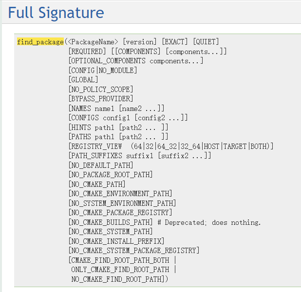
cmake的 find_package指令:
官方文档
find_package(包名 版本 REQUIRED)
一些包需要 sudo make install后才能被找到

LaTex
$\mathfrak{g}$
g \mathfrak{g} g
$\mathbb{R}$
R \mathbb{R} R
$\times$
× \times ×
$\varphi$
φ \varphi φ
$\Phi$
Φ \Phi Φ

$\overset{\mathrm{def}}{=}$
$\xlongequal{def}$
= d e f \overset{\mathrm{def}}{=} =def
= d e f \xlongequal{def} def