【Pytorch】深度学习之损失函数-编程知识

文章目录

二分类交叉熵损失函数
交叉熵损失函数
L1损失函数
MSE损失函数
平滑L1(Smooth L1)损失函数
目标泊松分布的负对数似然损失
KL散度
MarginRankingLoss
多标签边界损失函数
二分类损失函数
多分类的折页损失
三元组损失
HingEmbeddingLoss
余弦相似度
CTC损失函数
参考资料

学习目标：

二分类交叉熵损失函数

函数
torch.nn.BCELoss(weight=None, size_average=None, reduce=None, reduction='mean')
input为sigmoid函数的输出或softmax函数的输出
label为{0, 1}
功能：计算二分类任务时的交叉熵（Cross Entropy）
参数说明
weight：给每个类别的loss设置权值
size_average：bool类型，值为True时，返回各样本loss平均值；值为False时，返回各样本loss之和
reduce：bool类型，值为True时，返回loss为标量
代码说明

m = nn.Sigmoid()
loss = nn.BCELoss()
input = torch.randn(3, requires_grad=True)
target = torch.empty(3).random_(2)
output = loss(m(input), target)
output.backward()
print('BCELoss损失函数的计算结果为',output)

交叉熵损失函数

函数
torch.nn.CrossEntropyLoss(weight=None, size_average=None, ignore_index=-100, reduce=None, reduction='mean')
功能：计算交叉熵
计算公式
$-log(\frac{exp(x[class])}{\sum_jexp(x[j])}) = -x[class] + log(\sum_jexp(x[j]))$

loss = nn.CrossEntropyLoss()
input = torch.randn(3, 5, requires_grad=True)
target = torch.empty(3, dtype=torch.long).random_(5)
output = loss(input, target)
output.backward()

L1损失函数

函数
torch.nn.L1Loss(size_aveage=None, reduce=None, reduction='mean')
功能：output和真实标签之间差值的绝对值
参数说明
reduction参数——决定计算模式
none——逐个元素计算，output和输入元素同尺寸
sum——所有元素求和，返回标量
mean——加权平均，返回标量
计算公式
$L_n = |x_n-y_n|$
代码示例

loss = nn.L1Loss()
input = torch.randn(3, 5, requires_grad=True)
target = torch.randn(3, 5)
output = loss(input, target)
output.backward()

MSE损失函数

函数
torch.nn.MSELoss(size_average=None, reduce=None, reduction='mean')
功能：计算output和真实标签target之差的平方
代码示例

loss = nn.MSELoss()
input = torch.randn(3, 5, requires_grad=True)
target = torch.randn(3, 5)
output = loss(input, target)
output.backward()

平滑L1(Smooth L1)损失函数

torch.nn.SmoothLoss(size_average=None, reduce=None, reduction='mean', beta=1.0)
功能：L1损失函数的平滑输出，能够减轻离群点带来的影响
计算公式
$loss(x,y)=\frac{1}{n}\sum_{i=1}^nz_i$
其中， $z_i$ 的计算公式如下

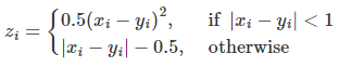
代码示例

loss = nn.SmoothL1Loss()
input = torch.randn(3, 5, requires_grad=True)
target = torch.randn(3, 5)
output = loss(input, target)
output.backward()

对比平滑L1和L1
可视化两种损失函数曲线

inputs = torch.linspace(-10, 10, steps=5000)
target = torch.zeros_like(inputs)loss_f_smooth = nn.SmoothL1Loss(reduction='none')
loss_smooth = loss_f_smooth(inputs, target)
loss_f_l1 = nn.L1Loss(reduction='none')
loss_l1 = loss_f_l1(inputs,target)plt.plot(inputs.numpy(), loss_smooth.numpy(), label='Smooth L1 Loss')
plt.plot(inputs.numpy(), loss_l1, label='L1 loss')
plt.xlabel('x_i - y_i')
plt.ylabel('loss value')
plt.legend()
plt.grid()
plt.show()

目标泊松分布的负对数似然损失

适用于回归任务，目标值（ground truth）服从泊松分布的回归问题，典型场景包括计数数据、连续型回归问题，如一天内发生的事件次数、网页访问次数
泊松分布： $\frac{\lambda^k}{k!}e^{-\lambda}$

torch.nn.PoissonNLLLoss(log_input=True, full=false, size_average=None, eps=1e-08, reduce=None, reduction='mean')
参数解释
log_input：bool类型参数，用于说明输入是否为对数形式
full：bool类型，是否计算所有loss
eps：修正项，用于避免input为0时，log(input)为Nan的情况
计算公式
当参数log_input=True： $loss(x_n, y_n)=e^{x_n}-x_n\cdot y_n$
当参数log_input=False： $loss(x_n, y_n) = x_n-y_n\cdot log(x_n+eps)$
代码示例

loss = nn.PoissonNLLLoss()
log_input = torch.randn(5, 2, requires_grad=True)
target = torch.randn(5, 2)
output = loss(log_input, target)
output.backward()

KL散度

torch.nn.KLDivLoss(size_average=None, reduce=None, reduction='mean', log_target=False)
功能：计算相对熵，度量连续分布的距离，对离散采用的连续输出空间分布进行回归
参数解释
reduction
取值有none/sum/mean/batchmean
none：逐个元素计算
sum：求和
mean：加权求和
batchmean：batchsize维度求平均值
计算公式

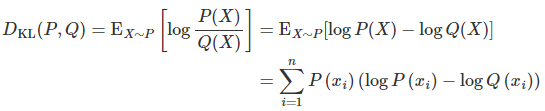
代码示例

inputs = torch.tensor([[0.5, 0.3, 0.2], [0.2, 0.3, 0.5]])
target = torch.tensor([[0.9, 0.05, 0.05], [0.1, 0.7, 0.2]], dtype=torch.float)
loss = nn.KLDivLoss()
output = loss(inputs,target)print('KLDivLoss损失函数的计算结果为',output)

MarginRankingLoss

torch.nn.MarginRankingLoss(margin=0.0, size_average=None, reduce=None, reduction='mean')
功能：计算两个向量之间的相似度，用于排序任务，又称为排序损失函数

参数解释
margin：边界值，两个向量之间的差异值
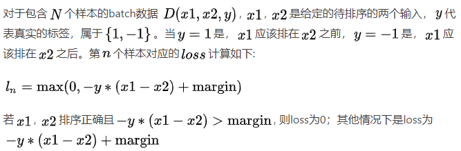
计算公式
$loss(x_1, x_2, y) = max(0, -y*(x_1-x_2)+margin)$
代码示例

loss = nn.MarginRankingLoss()
input1 = torch.randn(3, requires_grad=True)
input2 = torch.randn(3, requires_grad=True)
target = torch.randn(3).sign()
output = loss(input1, input2, target)
output.backward()print('MarginRankingLoss损失函数的计算结果为',output)

多标签边界损失函数

torch.nn.MultiLabelMarginLoss(size_average=None, reduce=None, reduction='mean')

关注的是样本和决策边界之间的间隔，使每个标签的得分都高于一个给定的阈值，并最小化样本与这些决策边界之间的间隔

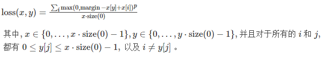
计算公式
$\frac{1}{N}\sum^N_{i=1}\sum^C_{j=1}L_{ij}$
其中，N为样本数量，C为标签数量， $L_{ij}$ 为样本i对标签j的边界损失
$L_{ij}=max(0, 1-y_{ij}\cdot f(x)_{ij})$
$y_{ij}$ 取值为 -1 或 1，表示标签 j 是否属于样本 i 的真实标签
若 $y_{ij}=1$ ，则要求 $f(x)_{ij} \geq margin$ ；若 $y_{ij}=-1$ ，则要求 $f(x)_{ij} \leq margin$

代码示例

loss = nn.MultiLabelMarginLoss()
x = torch.FloatTensor([[0.9, 0.2, 0.4, 0.8]])
# for target y, only consider labels 3 and 0, not after label -1
y = torch.LongTensor([[3, 0, -1, -1]])# 真实的分类是，第3类和第0类，标签中的-1表示该标签不适用于该样本
output = loss(x, y)print('MultiLabelMarginLoss损失函数的计算结果为',output)

二分类损失函数

torch.nn.SoftMarginLoss(size_average=None, reduce=None, reduction='mean')
功能：计算二分类的logistic损失，在训练SVM被经常使用，使得正确分类的样本得分与正确类别的边界之差大于一个预定义的边界值
计算公式
$f(x))=\frac{1}{N}\sum^N_{i=1}max(0, 1-y_{i}\cdot f(x)_{i})$
样本的真实标签和预测得分的乘积与1之差的最大值
若 $y_{i}\cdot f(x)_{i} \geq 1$ ，样本被正确分类，损失为0
反之，样本离正确分类还有距离，加入损失
代码示例

inputs = torch.tensor([[0.3, 0.7], [0.5, 0.5]])  # 两个样本，两个神经元
target = torch.tensor([[-1, 1], [1, -1]], dtype=torch.float)  # 该 loss 为逐个神经元计算，需要为每个神经元单独设置标签loss_f = nn.SoftMarginLoss()
output = loss_f(inputs, target)print('SoftMarginLoss损失函数的计算结果为',output)

多分类的折页损失

torch.nn.MultiMarginLoss(p=1, margin=1.0, weight=None, size_average=None, reduce=None, reduction='mean')
参数解释
p：可选 1 或 2
weight：各类别loss的权值
计算公式

代码示例

inputs = torch.tensor([[0.3, 0.7], [0.5, 0.5]]) 
target = torch.tensor([0, 1], dtype=torch.long) loss_f = nn.MultiMarginLoss()
output = loss_f(inputs, target)print('MultiMarginLoss损失函数的计算结果为',output)

三元组损失

torch.nn.TripletMarginLoss(margin=1.0, p=2.0, eps=1e-06, swap=False, size_average=None, reduce=None, reduction='mean')
说明
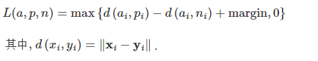
三元组：特殊的数据存储格式，有很多具体的引用，如nlp的关系抽取任务中<实体1，关系，实体2>，又如项目中的<anchor, positive examples, negative examples>
损失函数倾向于使anchor与positive examples的距离更近，而与negative examples的距离更远
计算公式

代码示例

triplet_loss = nn.TripletMarginLoss(margin=1.0, p=2)
anchor = torch.randn(100, 128, requires_grad=True)
positive = torch.randn(100, 128, requires_grad=True)
negative = torch.randn(100, 128, requires_grad=True)
output = triplet_loss(anchor, positive, negative)
output.backward()
print('TripletMarginLoss损失函数的计算结果为',output)

HingEmbeddingLoss

torch.nn.HingeEmbeddingLoss(margin=1.0, size_average=None, reduce=None, reduction='mean')
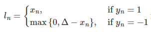
计算公式

代码示例

loss_f = nn.HingeEmbeddingLoss()
inputs = torch.tensor([[1., 0.8, 0.5]])
target = torch.tensor([[1, 1, -1]])
output = loss_f(inputs,target)print('HingEmbeddingLoss损失函数的计算结果为',output)

余弦相似度

torch.nn.CosineEmbeddingLoss(margin=0.0, size_average=None, reduce=None, reduction='mean')
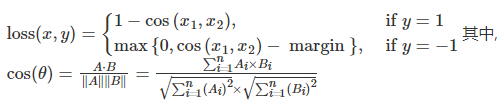
计算公式

代码示例

loss_f = nn.CosineEmbeddingLoss()
inputs_1 = torch.tensor([[0.3, 0.5, 0.7], [0.3, 0.5, 0.7]])
inputs_2 = torch.tensor([[0.1, 0.3, 0.5], [0.1, 0.3, 0.5]])
target = torch.tensor([1, -1], dtype=torch.float)
output = loss_f(inputs_1,inputs_2,target)print('CosineEmbeddingLoss损失函数的计算结果为',output)

CTC损失函数

CTC(Connectionist Temporal Classification)处理seq2seq任务，如语音识别、手写体识别，解决序列对齐问题，即在输入序列和目标序列长度不同的情况下，计算它们之间的对应关系
计算路径概率：对于给定的输入序列和目标标签，CTC损失考虑所有可能的对齐路径，在这些对齐路径对应的对齐方式中，重复字符被合并，空白标签被插入。CTC损失计算这些路径的概率之和
在反向传播中，CTC损失也会考虑所有可能的对齐方式

$\hat y) = -log(P(\hat y|y))$
torch.nn.CTCLoss(blank=0, reduction='mean', zero_infinity=False)
功能：用于时序类数据的分类，计算连续时间序列和目标序列之间的损失
参数解释
blank：blank label
zero_infinity：无穷大的值
代码示例

# Target are to be padded
T = 50      # Input sequence length
C = 20      # Number of classes (including blank)
N = 16      # Batch size
S = 30      # Target sequence length of longest target in batch (padding length)
S_min = 10  # Minimum target length, for demonstration purposes# Initialize random batch of input vectors, for *size = (T,N,C)
# 生成一批随机输入序列
# 这些input序列通过softmax函数沿着最后一个维度(detach函数)传递，对数化处理
input = torch.randn(T, N, C).log_softmax(2).detach().requires_grad_()# Initialize random batch of targets (0 = blank, 1:C = classes) 生成随机目标标签
target = torch.randint(low=1, high=C, size=(N, S), dtype=torch.long)# 初始化input序列长度和目标序列长度，input中每个序列长度都为样本最大序列长度T，target中每个序列长度为S_min到S之间的随机值
input_lengths = torch.full(size=(N,), fill_value=T, dtype=torch.long)
target_lengths = torch.randint(low=S_min, high=S, size=(N,), dtype=torch.long)
ctc_loss = nn.CTCLoss()
loss = ctc_loss(input, target, input_lengths, target_lengths)
loss.backward()

# Target are to be un-padded
T = 50      # Input sequence length
C = 20      # Number of classes (including blank)
N = 16      # Batch size# Initialize random batch of input vectors, for *size = (T,N,C)
input = torch.randn(T, N, C).log_softmax(2).detach().requires_grad_()
input_lengths = torch.full(size=(N,), fill_value=T, dtype=torch.long)# Initialize random batch of targets (0 = blank, 1:C = classes)
target_lengths = torch.randint(low=1, high=T, size=(N,), dtype=torch.long)
# target的生成方式变化，使用的是每个样本的长度来生成target
target = torch.randint(low=1, high=C, size=(sum(target_lengths),), dtype=torch.long)
ctc_loss = nn.CTCLoss()
loss = ctc_loss(input, target, input_lengths, target_lengths)
loss.backward()print('CTCLoss损失函数的计算结果为',loss)

关于seq2seq任务中的pading和unpadding：
填充：使所有序列达到相同的长度，以便进行批处理操作。通过在短序列两侧添加特殊标记（通常是0）来保持相同的长度。适用要求输入序列长度相同的模型，如循环神经网络（RNN）或卷积神经网络（CNN）等
不填充：模型可以直接根据输入序列的实际长度进行建模。适用于模型能够处理变长输入和目标序列的情况，如注意力机制（Attention Mechanism）或Connectionist Temporal Classification（CTC）损失