机器学习与深度学习——自定义函数进行线性回归模型
目的与要求
1、通过自定义函数进行线性回归模型对boston数据集前两个维度的数据进行模型训练并画出SSE和Epoch曲线图,画出真实值和预测值的散点图,最后进行二维和三维度可视化展示数据区域。
2、通过自定义函数进行线性回归模型对boston数据集前四个维度的数据进行模型训练并画出SSE和Epoch曲线图,画出真实值和预测值的散点图,最后进行可视化展示数据区域。
步骤
1、先载入boston数据集 Load Iris data
2、分离训练集和设置测试集split train and test sets
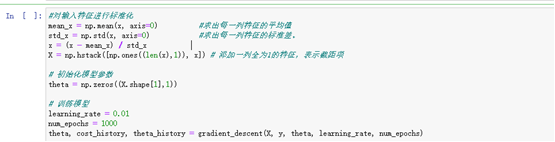
3、对数据进行标准化处理Normalize the data
4、自定义损失函数
5、使用梯度下降算法训练线性回归模型
6、初始化模型参数
7、训练模型
8、对训练集和新数据进行预测
9、画出SSE和Epoch折线图
10、画出真实值和预测值的散点图
11、进行可视化
代码
1、通过自定义函数进行线性回归模型对boston数据集前两个维度的数据进行模型训练并画出SSE和Epoch曲线图,画出真实值和预测值的散点图,最后进行二维和三维度可视化展示数据区域。
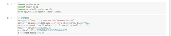
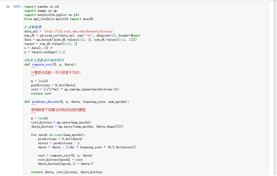
#引入所需库
import pandas as pd
import numpy as np
import matplotlib.pyplot as plt
from mpl_toolkits.mplot3d import Axes3D# 读取数据
data_url = "http://lib.stat.cmu.edu/datasets/boston"
raw_df = pd.read_csv(data_url, sep="\s+", skiprows=22, header=None)
data = np.hstack([raw_df.values[::2, :], raw_df.values[1::2, :2]])
target = raw_df.values[1::2, 2]
x = data[:,:2] # 只使用前两个特征进行线性回归
y = target.reshape(-1,1)#自定义函数进行线性回归
def compute_cost(X, y, theta):"""计算损失函数(平均误差平方和)"""m = len(y)predictions = X.dot(theta)cost = (1/(2*m)) * np.sum(np.square(predictions-y))return costdef gradient_descent(X, y, theta, learning_rate, num_epochs):"""使用梯度下降算法训练线性回归模型"""m = len(y)cost_history = np.zeros(num_epochs)theta_history = np.zeros((num_epochs, theta.shape[0]))for epoch in range(num_epochs):predictions = X.dot(theta)errors = predictions - ytheta = theta - (1/m) * learning_rate * (X.T.dot(errors))cost = compute_cost(X, y, theta)cost_history[epoch] = costtheta_history[epoch,:] = theta.Treturn theta, cost_history, theta_history#对输入特征进行标准化
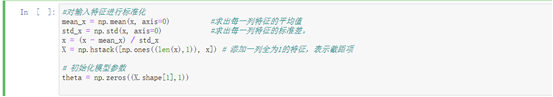
mean_x = np.mean(x, axis=0) #求出每一列特征的平均值
std_x = np.std(x, axis=0) #求出每一列特征的标准差。
x = (x - mean_x) / std_x #将每一列特征进行标准化,即先将原始数据减去该列的平均值,再除以该列的标准差,这样就能得到均值为0,标准差为1的特征
X = np.hstack([np.ones((len(x),1)), x]) # 添加一列全为1的特征,表示截距项# 初始化模型参数
theta = np.zeros((X.shape[1],1))# 训练模型
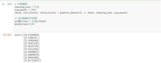
learning_rate = 0.01
num_epochs = 1000
theta, cost_history, theta_history = gradient_descent(X, y, theta, learning_rate, num_epochs)# 对训练集进行预测
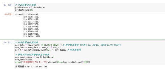
predictions = X.dot(theta)
predictions[:10]# 对新数据进行预处理
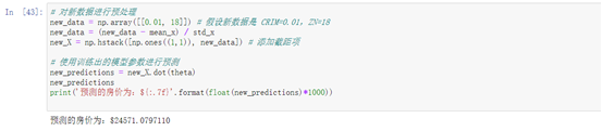
new_data = np.array([[0.01, 18]]) # 假设新数据是 CRIM=0.01,ZN=18
new_data = (new_data - mean_x) / std_x
new_X = np.hstack([np.ones((1,1)), new_data]) # 添加截距项# 使用训练出的模型参数进行预测
new_predictions = new_X.dot(theta)
new_predictions
print('预测的房价为:${:.7f}'.format(float(new_predictions)*1000))# 画出Epoch曲线图
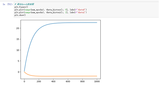
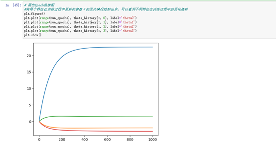
#将每个特征在训练过程中更新的参数θ的变化情况绘制出来,可以看到不同特征在训练过程中的变化趋势
plt.figure()
plt.plot(range(num_epochs), theta_history[:, 0], label='theta0')
plt.plot(range(num_epochs), theta_history[:, 1], label='theta1')
plt.show()# 画出SSE和Epoch折线图
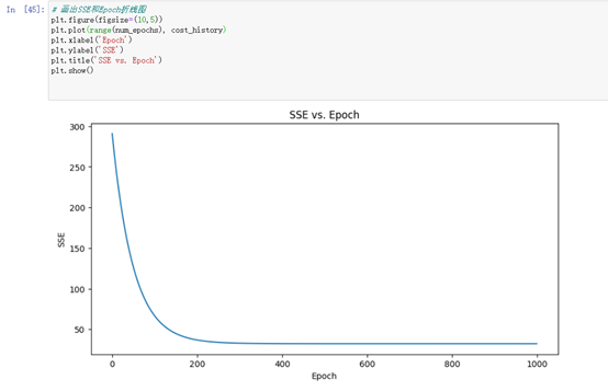
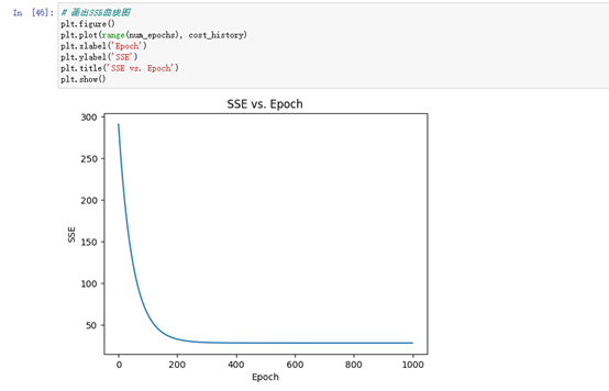
plt.figure(figsize=(10,5))
plt.plot(range(num_epochs), cost_history)
plt.xlabel('Epoch')
plt.ylabel('SSE')
plt.title('SSE vs. Epoch')
plt.show()# 画出预测值与真实值的比较图
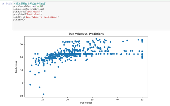
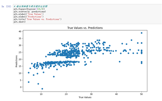
plt.figure(figsize=(10,5))
plt.scatter(y, predictions)
plt.xlabel('True Values')
plt.ylabel('Predictions')
plt.title('True Values vs. Predictions')
plt.show()# 画出数据二维可视化图
plt.figure(figsize=(10,5))
plt.scatter(x[:,0], y)
plt.xlabel('CRIM')
plt.ylabel('MEDV')
plt.title('CRIM vs. MEDV')
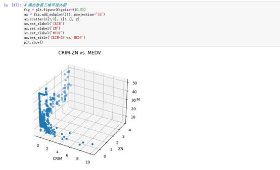
plt.show()# 画出数据三维可视化图
fig = plt.figure(figsize=(10,5))
ax = fig.add_subplot(111, projection='3d')
ax.scatter(x[:,0], x[:,1], y)
ax.set_xlabel('CRIM')
ax.set_ylabel('ZN')
ax.set_zlabel('MEDV')
ax.set_title('CRIM-ZN vs. MEDV')
plt.show()1、通过自定义函数进行线性回归模型对boston数据集前四个维度的数据进行模型训练并画出SSE和Epoch曲线图,画出真实值和预测值的散点图,最后进行可视化展示数据区域。
import pandas as pd
import numpy as np
import matplotlib.pyplot as plt
#载入数据
data_url = "http://lib.stat.cmu.edu/datasets/boston"
raw_df = pd.read_csv(data_url, sep="\s+", skiprows=22, header=None)
data = np.hstack([raw_df.values[::2, :], raw_df.values[1::2, :2]])
target = raw_df.values[1::2, 2]
x = data[:,:2]#前2个维度
y = target
import pandas as pd
import numpy as np
import matplotlib.pyplot as plt
from mpl_toolkits.mplot3d import Axes3D# 读取数据
data_url = "http://lib.stat.cmu.edu/datasets/boston"
raw_df = pd.read_csv(data_url, sep="\s+", skiprows=22, header=None)
data = np.hstack([raw_df.values[::2, :], raw_df.values[1::2, :2]])
target = raw_df.values[1::2, 2]
x = data[:,:4] #
y = target.reshape(-1,1)#自定义函数进行线性回归
def compute_cost(X, y, theta):"""计算损失函数(平均误差平方和)"""m = len(y)predictions = X.dot(theta)cost = (1/(2*m)) * np.sum(np.square(predictions-y))return costdef gradient_descent(X, y, theta, learning_rate, num_epochs):"""使用梯度下降算法训练线性回归模型"""m = len(y)cost_history = np.zeros(num_epochs)theta_history = np.zeros((num_epochs, theta.shape[0]))for epoch in range(num_epochs):predictions = X.dot(theta)errors = predictions - ytheta = theta - (1/m) * learning_rate * (X.T.dot(errors))cost = compute_cost(X, y, theta)cost_history[epoch] = costtheta_history[epoch,:] = theta.Treturn theta, cost_history, theta_history#对输入特征进行标准化
mean_x = np.mean(x, axis=0) #求出每一列特征的平均值
std_x = np.std(x, axis=0) #求出每一列特征的标准差。
x = (x - mean_x) / std_x #将每一列特征进行标准化,即先将原始数据减去该列的平均值,再除以该列的标准差,这样就能得到均值为0,标准差为1的特征
X = np.hstack([np.ones((len(x),1)), x]) # 添加一列全为1的特征,表示截距项# 初始化模型参数
theta = np.zeros((X.shape[1],1))# 训练模型
learning_rate = 0.01
num_epochs = 1000
theta, cost_history, theta_history = gradient_descent(X, y, theta, learning_rate, num_epochs)
# 画出Epoch曲线图
#将每个特征在训练过程中更新的参数θ的变化情况绘制出来,可以看到不同特征在训练过程中的变化趋势
plt.figure()
plt.plot(range(num_epochs), theta_history[:, 0], label='theta0')
plt.plot(range(num_epochs), theta_history[:, 1], label='theta1')
plt.plot(range(num_epochs), theta_history[:, 2], label='theta2')
plt.plot(range(num_epochs), theta_history[:, 3], label='theta3')
plt.show()# 对训练集进行预测
predictions = X.dot(theta)
predictions[:10]# 对新数据进行预处理
new_data = np.array([[ 0.01,18,2.310,0]]) # 假设新数据是 CRIM=0.01,ZN=18,INDUS=2.310,CHAS=0
new_data = (new_data - mean_x) / std_x
new_X = np.hstack([np.ones((1,1)), new_data]) # 添加截距项# 使用训练出的模型参数进行预测
new_predictions = new_X.dot(theta)
new_predictions
print('预测的房价为:${:.7f}'.format(float(new_predictions)*1000))
# 画出SSE曲线图
plt.figure()
plt.plot(range(num_epochs), cost_history)
plt.xlabel('Epoch')
plt.ylabel('SSE')
plt.title('SSE vs. Epoch')
plt.show()
# 画出预测值与真实值的比较图
plt.figure(figsize=(10,5))
plt.scatter(y, predictions)
plt.xlabel('True Values')
plt.ylabel('Predictions')
plt.title('True Values vs. Predictions')
plt.show()# 可视化前四个维度的数据
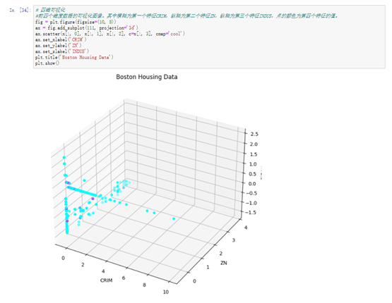
#前四个维度数据的可视化图像。其中横轴为第一个特征CRIM,纵轴为第二个特征ZN,纵轴为第三个特征INDUS,点的颜色为第四个特征的值。
fig = plt.figure(figsize=(10, 8))
ax = fig.add_subplot(111, projection='3d')
ax.scatter(x[:, 0], x[:, 1], x[:, 2], c=x[:, 3], cmap='cool')
ax.set_xlabel('CRIM')
ax.set_ylabel('ZN')
ax.set_zlabel('INDUS')
plt.title('Boston Housing Data')
plt.show()效果图
1、通过自定义函数进行线性回归模型对boston数据集前两个维度的数据进行模型训练并画出SSE和Epoch曲线图,画出真实值和预测值的散点图,最后进行二维和三维度可视化展示数据区域。

画出SSE(误差平方和)随Epoch(迭代次数)的变化曲线图,用来评估模型训练的效果。在每个Epoch,模型都会计算一次预测值并计算预测值与实际值之间的误差(即损失),然后通过梯度下降算法更新模型参数,使得下一次预测的误差更小。随着Epoch的增加,SSE的值会逐渐减小,直到收敛到一个最小值。

2、通过自定义函数进行线性回归模型对boston数据集前四个维度的数据进行模型训练并画出SSE和Epoch曲线图,画出真实值和预测值的散点图,最后进行可视化展示数据区域。
画出SSE(误差平方和)随Epoch(迭代次数)的变化曲线图,用来评估模型训练的效果。在每个Epoch,模型都会计算一次预测值并计算预测值与实际值之间的误差(即损失),然后通过梯度下降算法更新模型参数,使得下一次预测的误差更小。随着Epoch的增加,SSE的值会逐渐减小,直到收敛到一个最小值。
使用梯度下降算法训练线性回归模型的基本思路是:先随机初始化模型参数θ,然后通过迭代调整参数θ,使得损失函数的值尽量小。模型训练完成后,我们可以用训练好的模型对新的数据进行预测。