机器学习---比较单个学习器与Bagging集成的偏差-方差分解、在Iris数据集的不同特征子集上使用不同的分类器进行训练和可视化-编程知识

1. Bagging

说明并比较了预期均方误差的偏差方差分解，单个学习器与bagging集成的比较。

在回归中，估计器的预期均方误差可以根据偏差、方差和噪声进行分解。

在回归问题的数据集上的平均值上，偏差项测量估计器的预测与问题的最佳可能估计器（即贝叶斯

模型）的预测不同的平均量。

方差项测量在问题的不同实例上拟合时估计器的预测的可变性。

最后，噪声测量由于数据的可变性而导致的误差的不可约部分。

from sklearn.ensemble import BaggingClassifier
from sklearn.neighbors import KNeighborsClassifier
bagging = BaggingClassifier(KNeighborsClassifier(), max_samples=0.5, max_features=0.5)
import numpy as np
import matplotlib.pyplot as pltfrom sklearn.ensemble import BaggingRegressor
from sklearn.tree import DecisionTreeRegressor
# Settings
n_repeat = 50       # Number of iterations for computing expectations
n_train = 50        # Size of the training set
n_test = 1000       # Size of the test set
noise = 0.1         # Standard deviation of the noise
np.random.seed(0)
estimators = [("Tree", DecisionTreeRegressor()),("Bagging(Tree)", BaggingRegressor(DecisionTreeRegressor()))]n_estimators = len(estimators)

BaggingRegressor 和 DecisionTreeRegressor：分别是sklearn中的集成学习和决策树回归器。

estimators 是一个包含两个估算器的列表：

第一个是单个决策树回归器(DecisionTreeRegressor())。

第二个是使用Bagging方法包装的决策树回归器(BaggingRegressor(DecisionTreeRegressor()))。

Bagging通过对数据集进行自助采样（bootstrap）来构建多个子集合，然后对每个子集合进行训

练，最终将它们的预测进行平均或投票来得到最终结果。

# Generate data
def f(x):x = x.ravel() # ravel() 和 flatten()函数，将多维数组降为一维，ravel返回视图，flatten返回拷贝return np.exp(-x ** 2) + 1.5 * np.exp(-(x - 2) ** 2)# 生成符合真实世界数据分布的样本
def generate(n_samples, noise, n_repeat=1):# numpy.random.randn(d0, d1, …, dn)是从标准正态分布中返回一个或多个样本值。 # numpy.random.rand(d0, d1, …, dn)的随机样本位于[0, 1)中。 X = np.random.rand(n_samples) * 10 - 5X = np.sort(X)if n_repeat == 1:y = f(X) + np.random.normal(0.0, noise, n_samples) # numpy.random.normal(loc=0.0, scale=1.0, size=None) 均值，标准差，形状else:y = np.zeros((n_samples, n_repeat))for i in range(n_repeat):y[:, i] = f(X) + np.random.normal(0.0, noise, n_samples)X = X.reshape((n_samples, 1))return X, yX_train = []
y_train = []for i in range(n_repeat):X, y = generate(n_samples=n_train, noise=noise)X_train.append(X)y_train.append(y)X_test, y_test = generate(n_samples=n_test, noise=noise, n_repeat=n_repeat)plt.figure(figsize=(10, 8))

函数 f(x)：定义了一个简单的数学函数，根据输入的 x 返回一个相关的输出。使用指数函数和高斯

形状的组合来生成一个特定的模式。

函数 generate(n_samples, noise, n_repeat=1)：用于生成样本数据。它的作用是创建一个特定分

布模式的数据集。n_samples：生成的样本数量。noise：加入到数据中的噪声水平。n_repeat：

重复生成数据的次数。

首先，它生成 n_samples 个服从均匀分布的随机数 X，然后对其排序，从而得到 X。

对于单次生成（n_repeat = 1），它根据函数 f(x) 和指定的噪声水平 noise，生成对应的输出 y。

对于多次生成（n_repeat > 1），它为每次生成创建一个独立的输出 y，得到一个二维数组。

返回 X 和相应的 y。

数据生成和准备：使用 generate() 函数生成了 n_repeat 组训练数据，每组包含 n_train 个样本。

生成了一组包含 n_test 个样本的测试数据。

绘图准备：创建一个新的图形框架，设置图形大小为 10x8。

# Loop over estimators to compare
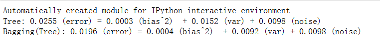
for n, (name, estimator) in enumerate(estimators):# Compute predictionsy_predict = np.zeros((n_test, n_repeat))for i in range(n_repeat):estimator.fit(X_train[i], y_train[i])y_predict[:, i] = estimator.predict(X_test)# Bias^2 + Variance + Noise decomposition of the mean squared errory_error = np.zeros(n_test)for i in range(n_repeat):for j in range(n_repeat):y_error += (y_test[:, j] - y_predict[:, i]) ** 2y_error /= (n_repeat * n_repeat)y_noise = np.var(y_test, axis=1)y_bias = (f(X_test) - np.mean(y_predict, axis=1)) ** 2y_var = np.var(y_predict, axis=1)print("{0}: {1:.4f} (error) = {2:.4f} (bias^2) "" + {3:.4f} (var) + {4:.4f} (noise)".format(name,np.mean(y_error),np.mean(y_bias),np.mean(y_var),np.mean(y_noise)))

循环遍历估算器：使用 enumerate(estimators) 枚举了估算器列表中的每个估算器，其中 name 是

估算器的名称，estimator 是对应的估算器对象。

计算预测值：为每个估算器，使用训练数据进行拟合，并在测试数据上进行预测。在这里，使用了

X_train[i] 和 y_train[i] 进行训练，然后用得到的模型 estimator 在 X_test 上进行预测。预测结果存

储在 y_predict 中。

计算均方误差的偏差-方差分解：偏差-方差分解是针对测试集上的每个样本进行的。

计算了模型预测误差的均方误差。这个误差是由三部分组成的：偏差的平方、方差和噪声。

y_error：初始化为全零数组，用来累加每个样本的误差。

通过两个嵌套循环计算每个样本的预测误差，并将其平均化，以得到均方误差。

计算了噪声的方差，通过 np.var(y_test, axis=1) 对测试集的输出值 y_test 沿着样本轴计算得到。

计算了偏差的平方，这里偏差定义为真实值 f(X_test) 与预测值的均值之差的平方。

计算了方差，表示模型预测的方差，通过对 y_predict 沿着样本轴计算得到。

将每个估算器的均方误差、偏差的平方、方差和噪声打印出来，以展示每个部分对于总误差的贡

献。打印的内容包括每个部分的平均值，以及其在总误差中的占比。

# Plot figuresplt.subplot(2, n_estimators, n + 1)plt.plot(X_test, f(X_test), "b", label="$f(x)$")plt.plot(X_train[0], y_train[0], ".b", label="LS ~ $y = f(x)+noise$")for i in range(n_repeat):if i == 0:plt.plot(X_test, y_predict[:, i], "r", label="$\^y(x)$")else:plt.plot(X_test, y_predict[:, i], "r", alpha=0.05)plt.plot(X_test, np.mean(y_predict, axis=1), "c",label="$\mathbb{E}_{LS} \^y(x)$")plt.xlim([-5, 5])plt.title(name)if n == n_estimators - 1:plt.legend(loc=(1.1, .5))plt.subplot(2, n_estimators, n_estimators + n + 1)plt.plot(X_test, y_error, "r", label="$error(x)$")plt.plot(X_test, y_bias, "b", label="$bias^2(x)$"),plt.plot(X_test, y_var, "g", label="$variance(x)$"),plt.plot(X_test, y_noise, "c", label="$noise(x)$")plt.xlim([-5, 5])plt.ylim([0, 0.1])if n == n_estimators - 1:plt.legend(loc=(1.1, .5))plt.subplots_adjust(right=.75)
plt.show()

设置子图和绘图：使用了 plt.subplot 来设置两行的子图布局，第一行展示了模型预测的情况，第二

行展示了误差、偏差、方差和噪声的分解情况。

第一个 plt.subplot 绘制了模型预测结果：绘制了真实函数 f(x) 的曲线。绘制了单次生成的训练数据

点，带有噪声。

对于每个重复的训练，绘制了模型在测试数据上的预测结果，这些结果用红色曲线表示。

绘制了所有模型预测的平均结果，用青色曲线表示。设置了横坐标范围为 -5 到 5。

给每个子图添加了标题和图例。第二个 plt.subplot 绘制了误差的偏差-方差分解结果：

绘制了预测误差（红色曲线）、偏差的平方（蓝色曲线）、方差（绿色曲线）和噪声（青色曲

线）。设置了横坐标范围为 -5 到 5，纵坐标范围为 0 到 0.1。添加了图例。

调整布局并展示图表：使用 plt.subplots_adjust(right=.75) 调整了子图布局，确保图例有足够的空

间。最后使用 plt.show() 展示了绘制好的图表。

2. 随机森林

#  Random Forests
from sklearn.ensemble import RandomForestClassifier
X = [[0, 0], [1, 1]]
Y = [0, 1]
clf = RandomForestClassifier(n_estimators=10)
clf = clf.fit(X, Y)
# Extremely Randomized Trees
from sklearn.model_selection import cross_val_score
from sklearn.datasets import make_blobs
from sklearn.ensemble import RandomForestClassifier
from sklearn.ensemble import ExtraTreesClassifier
from sklearn.tree import DecisionTreeClassifier
X, y = make_blobs(n_samples=10000, n_features=10, centers=100, random_state=0)
clf = DecisionTreeClassifier(max_depth=None, min_samples_split=2, random_state=0)
scores = cross_val_score(clf, X, y)
print(scores.mean())clf = RandomForestClassifier(n_estimators=10, max_depth=None, min_samples_split=2, random_state=0)
scores = cross_val_score(clf, X, y)
print(scores.mean())                     clf = ExtraTreesClassifier(n_estimators=10, max_depth=None, min_samples_split=2, random_state=0)
scores = cross_val_score(clf, X, y)
print(scores.mean() > 0.999)

随机森林与极端随机树的分类：

导入了 RandomForestClassifier、ExtraTreesClassifier 和 DecisionTreeClassifier 等分类器。

首先，使用一个简单的例子 X = [[0, 0], [1, 1]] 和 Y = [0, 1] 对随机森林模型进行了训练和拟合。

接着，创建了一个更复杂的数据集 make_blobs，其中包含了 10000 个样本、10个特征、100个中

心点，这是一个用于分类的合成数据集。

评估模型性能：

对比了单个决策树、随机森林和极端随机树在这个合成数据集上的性能。

对单个决策树进行了交叉验证评分，并打印了其平均分数。

对随机森林和极端随机树分别进行了交叉验证评分，并打印了它们的平均分数。

最后，打印了极端随机树的平均分数是否大于0.999（如果是，则打印True，否则打印False）。

import numpy as np
import matplotlib.pyplot as plt
from matplotlib.colors import ListedColormapfrom sklearn import clone
from sklearn.datasets import load_iris
from sklearn.ensemble import (RandomForestClassifier, ExtraTreesClassifier,AdaBoostClassifier)
from sklearn.tree import DecisionTreeClassifier# Parameters
n_classes = 3
n_estimators = 30
cmap = plt.cm.RdYlBu
plot_step = 0.02  # fine step width for decision surface contours
plot_step_coarser = 0.5  # step widths for coarse classifier guesses
RANDOM_SEED = 13  # fix the seed on each iteration# Load data
iris = load_iris()plot_idx = 1models = [DecisionTreeClassifier(max_depth=None),RandomForestClassifier(n_estimators=n_estimators),ExtraTreesClassifier(n_estimators=n_estimators),AdaBoostClassifier(DecisionTreeClassifier(max_depth=3),n_estimators=n_estimators)]

参数设置：n_classes：类别数量，这里是鸢尾花数据集有3个类别。n_estimators：用于集成模型

的基础分类器数量。cmap：颜色映射，用于可视化不同类别的颜色。plot_step 和

plot_step_coarser：用于绘制决策边界的步长设置。RANDOM_SEED：随机种子，用于确保每次

迭代结果的一致性。

加载数据：使用 load_iris() 加载了鸢尾花数据集。

模型准备：创建了一个包含不同分类器的列表 models，包括：DecisionTreeClassifier：单个决策

树分类器。RandomForestClassifier：随机森林分类器。ExtraTreesClassifier：极端随机树分类

器。AdaBoostClassifier：AdaBoost分类器，基础分类器为决策树，最大深度为3。

循环遍历特征子集和模型：通过循环迭代每个特征子集和每个模型，以不同的特征组合训练不同的

模型。对于每个模型，首先选择了一个特征子集，然后对数据进行随机化和标准化。对模型进行拟

合，并计算其在训练集上的准确率。绘制了决策边界，展示了每个模型在不同特征子集上的分类情

况和区分能力。

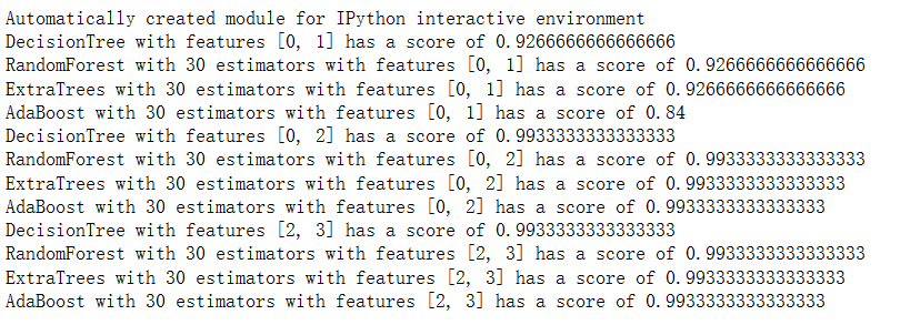
for pair in ([0, 1], [0, 2], [2, 3]):for model in models:# We only take the two corresponding featuresX = iris.data[:, pair]y = iris.target# Shuffleidx = np.arange(X.shape[0])np.random.seed(RANDOM_SEED)np.random.shuffle(idx)X = X[idx]y = y[idx]# Standardizemean = X.mean(axis=0)std = X.std(axis=0)X = (X - mean) / std# Trainclf = clone(model)clf = model.fit(X, y)scores = clf.score(X, y)# Create a title for each column and the console by using str() and# slicing away useless parts of the stringmodel_title = str(type(model)).split(".")[-1][:-2][:-len("Classifier")]model_details = model_titleif hasattr(model, "estimators_"):model_details += " with {} estimators".format(len(model.estimators_))print(model_details + " with features", pair,"has a score of", scores)plt.subplot(3, 4, plot_idx)if plot_idx <= len(models):# Add a title at the top of each columnplt.title(model_title)# Now plot the decision boundary using a fine mesh as input to a# filled contour plotx_min, x_max = X[:, 0].min() - 1, X[:, 0].max() + 1y_min, y_max = X[:, 1].min() - 1, X[:, 1].max() + 1xx, yy = np.meshgrid(np.arange(x_min, x_max, plot_step),np.arange(y_min, y_max, plot_step))# Plot either a single DecisionTreeClassifier or alpha blend the# decision surfaces of the ensemble of classifiersif isinstance(model, DecisionTreeClassifier):Z = model.predict(np.c_[xx.ravel(), yy.ravel()])Z = Z.reshape(xx.shape)cs = plt.contourf(xx, yy, Z, cmap=cmap)else:# Choose alpha blend level with respect to the number# of estimators# that are in use (noting that AdaBoost can use fewer estimators# than its maximum if it achieves a good enough fit early on)estimator_alpha = 1.0 / len(model.estimators_)for tree in model.estimators_:Z = tree.predict(np.c_[xx.ravel(), yy.ravel()])Z = Z.reshape(xx.shape)cs = plt.contourf(xx, yy, Z, alpha=estimator_alpha, cmap=cmap)# Build a coarser grid to plot a set of ensemble classifications# to show how these are different to what we see in the decision# surfaces. These points are regularly space and do not have a# black outlinexx_coarser, yy_coarser = np.meshgrid(np.arange(x_min, x_max, plot_step_coarser),np.arange(y_min, y_max, plot_step_coarser))Z_points_coarser = model.predict(np.c_[xx_coarser.ravel(),yy_coarser.ravel()]).reshape(xx_coarser.shape)cs_points = plt.scatter(xx_coarser, yy_coarser, s=15,c=Z_points_coarser, cmap=cmap,edgecolors="none")# Plot the training points, these are clustered together and have a# black outlineplt.scatter(X[:, 0], X[:, 1], c=y,cmap=ListedColormap(['r', 'y', 'b']),edgecolor='k', s=20)plot_idx += 1  # move on to the next plot in sequenceplt.suptitle("Classifiers on feature subsets of the Iris dataset")
plt.axis("tight")plt.show()

循环特征子集和模型：外部循环遍历了三个不同的特征子集 ([0, 1], [0, 2], [2, 3])，即每次只选择两

个特征来进行训练和可视化。内部循环遍历了不同的模型列表 models，对每个特征子集使用每个

模型进行训练和绘图。

数据准备和模型训练：对于每个特征子集和每个模型，首先从鸢尾花数据集中选择相应的特征和目

标变量。对数据进行随机化和标准化，然后使用 clone() 复制模型，并训练模型。计算模型在训练

集上的准确率，并打印每个模型的类型及对应特征子集的得分。

绘制决策边界：使用 plt.subplot() 设置子图，并对每个模型在不同特征子集上进行可视化。

绘制了决策边界，使用填充轮廓图 (plt.contourf()) 来表示模型的分类决策。

对于单个决策树，绘制了单一的决策边界；对于集成模型，利用每个基本分类器的预测结果进行

alpha 混合，绘制了决策边界。

可视化结果：在子图中展示了每个模型在不同特征子集上的决策边界图。在图中通过散点图展示了

训练数据点，不同类别使用不同颜色表示。