Summerize for Bioinformatics with ChatGPT-编程知识

Basic Introduction

Historical Events

Bioinformatics vs. Computational Biology

Levels of Bioinfo & CompBio

Molecular Biology Primer

Homework 1

A brief Introduction to DNA & RNA

A brief Introduction to Protein

Sequencing Technologies

Sequence Alignment

Pairwise sequence alignment

Basic notions

Goal of Pairwise Alignment:

Algorithms for G&L Alignments

Homework 2

Database similarity searches

BLAST: Basic Local Alignment Search Tool

FASTA: FAST-All

Comparison between BLAST & FASTA

Homework 3

Multiple sequence alignment

1. Progressive alignment methods

2. Iterative alignment methods

PSSM方法

Motifs and domains

Homework 4

My understanding to Expectation Maximization(EM) Algorithm:

Core Algorithm:

Code in PyCharm: (python=3.8)

The final result:

The difficulties I met:

Machine Learning Approaches

GA for sequencing and MSA

Sequencing by Using GA

Multiple Sequence Alignments Using GA

Protein Function Prediction

Gene Function Prediction Using SVM

Protein Function Prediction Using DNN

Protein Structure Prediction

Protein Folding Based on EDA

Protein Folding Based on Deep Reinforcement Learning

AlphaFold2 for Protein Structure Prediction

References

Basic Introduction

Historical Events

Bioinformatics vs. Computational Biology

Bioinformatics = the creation of tools (algorithms, databases) that solve problems. The goal is to build useful tools that work on biological data. lt is about engineering.
Computational biology = the study of biology using computational techniques. The goal is to learn new biology, knowledge about living systems. lt is about discovery.

Levels of Bioinfo & CompBio

Level 0: Modeling for modeling's sake
Level 1: (entry) Use published tools to analyze data and generate hypotheses for experimentalists
Level 2 (Bioinfo): Develop algorithms and databases for data analyses on new technologies, data integration and reuse.
Level 3 (CompBio): Make biological discoveries from public dataintegration and modeling
Level X: Integrative studies from big consortia

Molecular Biology Primer

All life depends on 3 critical molecules

DNAs

Hold information on how cell works

RNAs

Act to transfer short pieces of information to different parts of cell

Provide templates to synthesize into protein

Proteins

Form enzymes(酶) that send signals to other cells and regulate gene activity

Form body’s major components (e.g. hair, skin, etc.)

蛋白质在生命系统中的重要作用：

• Catalysis催化作用

• Carrier and transport承运人和运输

• Regulatory调节

Homework 1

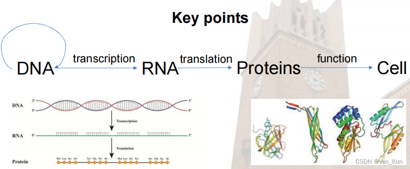
Write a report describing Cell, DNA, RNA, Proteins and discussing their relations, from information point of view.

Replication: 复制
Transcription: 转录
Translation: 翻译

A brief Introduction to DNA & RNA

DNA & RNA are polymers(聚合物) of nucleotides(核苷酸)
- DNA is a nucleic acid, made of long chains of nucleotides, which has four kinds of bases, A, T, C, G. DNA is a double strand helix(双链螺旋), hydrogen bonds(氢键) between bases(碱基) hold the strands together: A and T, C and G.
  - Untwisting and replication (using DNA polymerase(聚合酶)): each strand is a template of a new strand
  - DNA replication begins at many specific sites
  - Each strand of the double helix is oriented in the opposite direction
  - The sequence of codons in DNA spells out the primary structure of a polypeptide
    
    (Polypeptides form proteins that cells and organisms use)
- RNA is also a nucleic acid: different sugar (has 1 more O on the 2nd Carbon) ; U instead of T; Single strand, usually

A brief Introduction to Protein

Proteins are key players in our living systems.
Proteins are polymers consisting of 20 kinds of amino acids. (没有BJOUXZ这六个字母)
Each protein folds into a unique three-dimensional structure defined by its amino acid sequence.
Protein structure has a hierarchical nature(层级性).
Protein structure is closely related to its function.
Protein structure prediction is a grand challenge of computational biology

Sequencing Technologies

1st gen: Sanger sequencing (桑格测序)

DNA片段制备： 复制要测序的DNA片段。

反应混合物： 创建一个反应混合物，其中包括标准核苷酸（A、T、C、G）和一小部分双脱氧核苷酸（ddATP、ddTTP、ddCTP、ddGTP）。

DNA合成： 进行DNA合成反应，当DNA链生长到带有dideoxynucleotide（双脱氧核苷酸）的位置时，DNA链终止。

分离DNA片段： 通过凝胶电泳分离不同长度的DNA片段。

电泳分析： 分离的DNA片段形成带状图谱，根据其长度可视化。

结果解读： 通过分析图谱中的颜色或信号，确定DNA序列。

2nd gen: Illumina sequencing (伊卢米纳测序)

文库制备： 剪切DNA成短片段，添加适配器形成文库。

文库扩增： 扩增成数百万复制。

聚类： 形成DNA片段簇。

桥PCR： 将DNA片段桥接到适配器上。

测序： 逐一添加核苷酸，观察荧光信号，确定DNA序列。

数据分析： 处理图像和信号，得到原始测序数据。

序列拼接和分析： 将短读段拼接成完整序列，进行进一步的生物信息学分析。

3rd gen: Third generation sequencing (第三代测序)

DNA准备： 提取DNA并进行质控，确保适合直接测序。

DNA模板制备： 将DNA片段固定在SMRT细胞中，形成单分子的DNA模板。

SMRT细胞测序： 使用聚合酶在DNA模板上合成互补链，同时测量逐个核苷酸的加入，形成实时的荧光信号。

数据采集： 通过监测SMRT细胞中的DNA合成过程，实时获取长读长的测序数据。

数据分析： 对得到的原始数据进行处理和分析，包括错误校正和序列拼接。

Sequence Alignment

Pairwise sequence alignment

Basic notions

To express the relatedness:

identity 相同度
similarity 相似度（相似物化性质，可以被替换的碱基）
1. Calculation 1: $\frac{2*L_{s}}{L_{a}+L_{b}}$ (Ls: 相同/相似残基对数；La/Lb: 两条序列的长度)
2. Calculation 2: $\frac{L_{s}}{L_{a}}$ (Ls: 相同/相似残基对数；La: 较短序列的长度)
homology 同源性（序列间存在进化关系的推断）
1. Caution：同源性要么有要么没有，不能“有点”同源性！
2. Judgement：相同度和相似度的百分比（序列较短时会出现偶然）
  1. Solve：
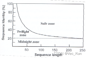
  2. （↑在Safe Zone里就可以安全地认为它是同源的）

Amino acids varies from "R" groups.

Amino acids are joined by amide linkages (酰胺键) to form proteins.
Each C-N bond is called a peptide bond (肽键).

A short chain of amino acids is called a peptide (多肽) (usually <100).
A longer chain of amino acids is called a protein.
When an amino acid is part of a peptide or protein, it is called an amino acid residue (残基).

amino terminus / N-terminus (氨基) , has a free amino group.

Residues are numbered at the beginning of N terminus.

carboxyl terminus / C-terminus (羧基) , has a free carboxyl group.

Goal of Pairwise Alignment:

Find best pairing of two sequences so there is maximum correspondence between residues.

Methods:

Global Alignment: 找到最适合于两个长度大致相同的高度相似的序列
Local Alignment: 找到两个序列相似性最高的区域，这两个序列的长度可以非常不同

Algorithms for G&L Alignments

1. Dot matrix (dot plot) method: 一种使用二维矩阵的图形化方法

构建矩阵： 将两个序列分别放置在矩阵的水平和垂直方向上，形成一个二维矩阵。

相似性标记： 在相同位置上，如果两个序列的字符相同或相似，就在该位置上绘制一个点（或其他符号）。

可视化： 查看绘制的点阵，观察序列之间的相似性模式。

2. ⭐ Dynamic programming (DP) method : 生成一个包含所有可能对齐的分数的二维对齐矩阵，以便定量地找到最佳对齐

需要一个评分方法（Scoring System）：

$score(A) = \alpha w- \beta x - \gamma y$

w: 配对数；x: 未配对数；y: 间隙（gap）数

Reward for matches: α (positive score)

Mismatch penalty: -β (negative score)

Gap penalty: -γ (negative score)

Global alignment: Needleman-Wunsch (NW) algorithm
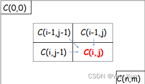
定义状态： 将比对问题划分为一个二维矩阵，矩阵的每个元素对应于两个序列的某一对字符。矩阵中的每个元素表示在该位置上的比对分数，即对应字符的相似性得分。

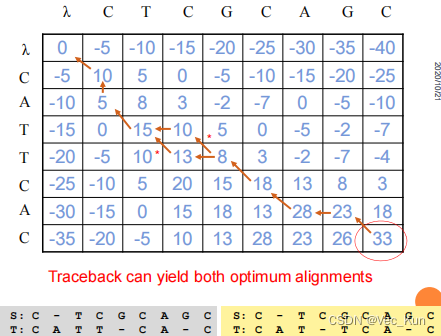
初始化： 在矩阵的第一行和第一列中设置初始值，表示第一个序列或第二个序列与空序列之间的比对分数。这些初始值是根据所选择的比对得分规则确定的。C(i,0)=-i*γ C(0,j)=-j*γ

状态转移方程： 确定状态之间的转移关系，即如何从先前的状态得到当前状态。在NW算法中，状态转移方程通常包括匹配、插入和删除操作，对应于在两个序列中移动、匹配或插入缺失字符。

w(a,b)=+α(if a=b)/-β(if a≠b)

For 1≤i≤n,1≤j≤m:
C(i,j)=max{ [C(i-1, j-1)+w(Si,Tj)], [C(i-1, j)-γ], [C(i, j-1)-γ]}
Si/Tj: Prefix of length i of S/T sequence

计算矩阵： 根据状态转移方程，计算整个矩阵的值。这可以通过自底向上的方式，从左上角逐步计算到右下角，也就是从序列的开头到末尾。

回溯： 根据计算得到的矩阵，从右下角开始回溯，找到最优比对路径。这个路径就是使两个序列得分最高的比对方式。时间复杂度O(mn)

Local alignment: Smith-Waterman (SW) algorithm
定义状态： 将比对问题划分为一个二维矩阵，矩阵的每个元素对应于两个序列的某一对字符。矩阵中的每个元素表示在该位置上的比对分数，即对应字符的相似性得分。(蛋白质局部相似可能对应着“功能亚基”相似，这是主要的)

初始化： 在矩阵的第一行和第一列中设置初始值为零，表示起始位置。与Needleman-Wunsch算法不同，Smith-Waterman算法的初始化值为零，不考虑与空序列的比对。

状态转移方程： 确定状态之间的转移关系，即如何从先前的状态得到当前状态。在SW算法中，状态转移方程包括匹配、插入、删除操作，对应于在两个序列中移动、匹配或插入缺失字符。

C(i,j)=max{ [C(i-1, j-1)+score(Si,Tj)], [C(i-1, j)-γ], [C(i, j-1)-γ], 0 }

计算矩阵： 根据状态转移方程，计算整个矩阵的值。这可以通过自底向上的方式，从左上角逐步计算到右下角，也就是从序列的开头到末尾。

回溯： 根据计算得到的矩阵，找到矩阵中的最高得分及其位置。从该位置开始回溯，沿着得分最高的路径，找到最优的局部比对。时间复杂度O(mn)

Gap Panalty Function (间隙惩罚函数)

Gap penalty = h + gk

where k = length of gap; h = gap opening penalty; g = gap continuation penalty （g＜h, 因为随着缺口开放会有几个残基伴随着插入或删除，所以应该减少额外残基的惩罚）

惩罚分数要合理：太高会导致没有空隙从而没有合理的对齐；太低会导致间隙太多让不相关的序列以高分对齐。

Substitution Matrix or Scoring Matrix （替代矩阵/评分矩阵）

PAM矩阵（Point Accepted Mutation）： 用于描述蛋白质的氨基酸替代概率（全局比对）。

BLOSUM矩阵（BLOcks SUbstitution Matrix）： 用于比对蛋白质序列。BLOSUM矩阵的版本如BLOSUM62常用于蛋白质序列比对（局部比对）。

DNA矩阵： 用于比对DNA序列，通常包括不同碱基之间的替代得分。

Extreme Value Distribution (极值分布)

生成分布： (例)通过对1000次与1000个随机打乱的序列进行比对，得到了一个包含1000个比对得分的分布。这个分布被称为Extreme Value Distribution。

绘制图表： 利用这1000个比对得分，制作了一个图表。通过观察图表，可以看出比对得分的整体分布模式，即极值分布的特定模式。

比对原始得分： 将原始的比对得分（S）与极值分布进行比对。如果原始得分（S）位于分布的极右边缘，那么说明该比对结果很可能不是由于随机情况而产生的，而是由于序列的同源性。

计算P-value： 通过极值分布的公式 $P(X\geq S)=1-e^{-Kmne^{\lambda S}}$ 计算P-value。（m和n是序列长度，K和λ是基于评分矩阵的常数）P-value表示原始比对得分出现在或更极端的位置的概率。P-value越小，说明比对不太可能是由于随机情况而产生的，从而增加了对同源性的推断的可信度。

3. Word method

Introduced in " Database similarity searches"

"word method" 可能指代对生物序列中的k-mer (一个 k-mer 是指长度为 k 的子串) 进行处理和分析的方法。

Homework 2

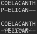
1. There are two amino acid sequences, seq1: COELACANTH and seq2: PELICAN. Obtain the global alignment by using DP (the Needleman-Wunsch algorithm) .

2. Two different dot matrix analysis servers to analyze the sequence of the human low density lipoprotein receptor(np_000518)

1. https://www.ncbi.nlm.nih.gov/protein/NP_000518.1 get the origin

2. https://www.ebi.ac.uk/Tools/seqstats/emboss_dottup/ generate the result

3. https://www.bioinformatics.nl/cgi-bin/emboss/dotmatcher generate the result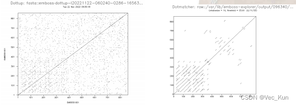

The long diagonal indicates that there exists a perfect match from the beginning to the end between the two sequences. (Because the two sequences are the same.)

The shorter diagonals represent the local approximate matches between the two sequences. The reason that those shorter diagonals mostly occur in the lower left corner is that there are many similar patterns before the position of 400.

Database similarity searches

" An application of Pairwise Sequence Alignment"

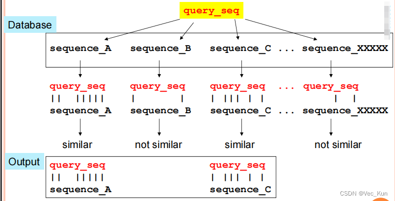
The basic procedure for doing this:

Submit the sequence of interest (the“query” sequence)
It is aligned in a pairwise manner to EVERY sequence in the database
Based on these pairwise comparisons, all sequences that have similarity to the query are found
Pairwise alignments between the query and each of these similar sequences are returned as output

Requirements: （尝试让这三者达到平衡，因为是相互掣肘的）

1. sensitivity (漏判越少敏感性越好)

2. specificity(selectivity) (误判越少特异性越好)

3. speed (从数据库搜索获取输出所需的时间越少速度越快)

Idea: 动态规划是穷举算法，时间效率低，在不影响太多敏感性和特异性的条件下，我们可以采用启发式算法(Heuristic Algorithms), but 不能保证找到最优/最准确的结果

Shortcut: “Test” each sequence to see whether it is worth aligning with query_seq

常见的启发式算法：BLAST 和 FASTA 它们就是所谓的WORD METHOD

Merits： 50-100 times faster than DP
Shorts：not guaranteed to find the best/most accurate result

Based on finding short stretches of identical or nearly identical letters (which are called “words”, “k-tuples ”, or “ ktups ”) in two sequences.

基本过程：

寻找相同的word(s)： 找到两个序列中共有的word或词组，并对它们进行比对。

通过对齐word扩展比对： 通过对齐每个word两侧的相似区域，扩展比对的范围。

计算对齐区域的得分： 对扩展后的对齐区域进行得分计算，通常使用某种评分矩阵或得分规则来衡量相似性。

连接高分区域： 将相邻的高分对齐区域连接在一起，形成最终的局部比对结果。

BLAST: Basic Local Alignment Search Tool

局部比对： BLAST采用局部比对的策略，即先寻找两个序列之间的局部相似性，然后根据这些局部相似性进行进一步的分析。

查询序列： 用户提供一个查询序列，可以是DNA、RNA或蛋白质序列。

数据库搜索： BLAST将查询序列与目标数据库中的序列进行比对。以蛋白质为例，一个长度为三的蛋白质单词要与20*20*20=8000个词比对。

比对算法： BLAST使用启发式算法，通过构建短词（words）的索引来加速搜索。它首先找到与查询序列中的短词相匹配的目标序列，然后通过局部比对的方式逐步扩展匹配区域。单词长度蛋白质通常是3个，DNA通常是11个

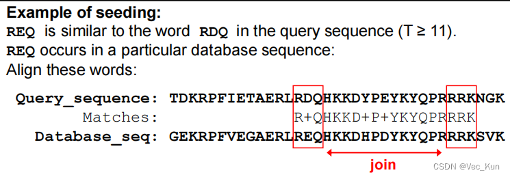
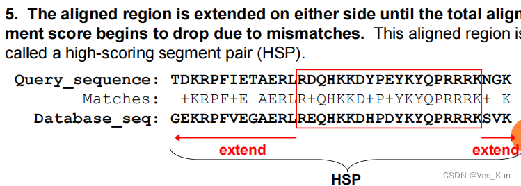
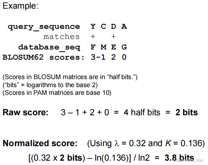
计算分数： BLAST根据相似性得分（根据选择的替代矩阵，例如BLOSUM或PAM矩阵）对匹配区域进行打分，默认是BLOSUM62。一般比对阈值(threshold)是T=11. 如果超过了阈值，那么就认为可以被替换，作为"seed", 例如下图：

如果在这个配对附近又出现了配对，可以将它们连接起来形成一段更长的无间隔的配对（早期BLAST不会这样）

基于这个配对序列，继续向两边扩展，直到分数开始下降，最终得到的就是HSP(高分段配对)

HSP分数大于某截断值(cutoff value)S时保留，否则丢弃；

单个数据库找到多个HSP就连接起来形成有缺口的配对（早期BLAST不会这样）

最后给查询序列和配对序列进行SW配对，配对的数据库序列称为“命中(hits)”查询序列

输出结果： BLAST输出匹配的序列及其相似性得分，同时提供了可视化的比对图形和其他有关匹配的信息。

P-value： BLAST的输出中通常包括P-value，表示在随机情况下得到相同或更好匹配的期望次数。P-value越小，表示匹配越显著。(We have mentioned this in the SW algorithm part)

注意：实际上m、n的定义变化了，在这里它们指的都是有效值，都是用实际长度减去两个对齐序列的对齐长度的平均值

E-value：Expected Value指的是the number of high-scoring matches we expect to observe between the query and unrelated sequences. 计算公式如下

D: 数据库里序列数目（数据库的大小size）

p: 根据极值分布，获得对齐得分≥S的概率

m’: 数据库的有效长度（数据库大小的另一种度量）

The E-value is the number of HSP’s with an alignment score ≥ S that are expected to occur by chance when searching a database of D sequences.

"The smaller the E-value, the less likely the alignment is due to chance"

搜索某一个数据库获得的E值不能用于其他数据库，因为数据库大小越大，E值更倾向于越大。

"A p-value is a way of representing the significance of an alignment. An E-value is simply another way of representing the significance of that alignment."

The normalization of scores: 对齐的原始分数取决于评分矩阵和间隙惩罚，而标准化分数可以独立于评分矩阵来评估不同BLAST查询得出的结果来判断哪个对齐更合理。

计算公式

S = raw alignment score 原始对齐分数； λ = constant that depends on scoring matrix 评分矩阵给出的常数； K = constant that depends on scoring matrix 评分矩阵给出的常数

LCR: Low Complexity Regions：低复杂度区域，信息重复且单一，都是短而重复的片段，会干扰最终输出的配对片段，在蛋白质序列中占约15%，可能会导致虚假命中和虚高配对分数（spurious hits and artificially high alignment scores）。

Avoid method 1: Filtering. 在查询区域把 LCR片段用小写字母或歧义字符替换（ 蛋白质X，DNA是N），当然这么做可能会遗漏一些真实匹配

Avoid Method 2: Masking. LCR中的字符在构建查询单词表中被忽略，但是可以在扩展和对齐优化中使用

FASTA: FAST-All

开发者： 由 David Lipman 和 William Pearson 于 1988 年开发。

首个广泛使用的快速数据库搜索程序： FASTA 是第一个被广泛使用的用于进行快速数据库搜索的程序。它的主要目的是在大型生物数据库中快速找到与查询序列相似的序列。

启发式词法方法： FASTA 使用一种启发式的 word 方法来创建查询序列与数据库序列之间的局部比对。该方法通过寻找两个序列中的词（words）的相似性来进行比对。

从精确匹配的词开始： FASTA 在比对过程中从寻找两个序列中的词的精确匹配开始。在蛋白质序列中，通常使用 ktup = 1 或 2，而在DNA序列中，通常使用 4-6。

Comparison between BLAST & FASTA

• BLAST is faster

• FASTA generally produces a better final alignment

• FASTA is more likely to find distantly related sequences

• Performance of the two methods is similar for highly similar sequences

• Both methods are appropriate for rapid initial searches

Homework 3

1. Answer the following questions about scoring an alignment.

A. Calculate the score for the DNA sequence alignment shown below, using the scoring matrix below. Use an affine gap penalty to score the gaps, with -11 for opening the gap and -1 for each additional position in the gap. (“Affine gap penalty” refers to a situation when the gap opening and gap extension penalties are not the same. The gap opening penalty should be greater than the gap extension penalty.)

2x27–5x4–11–2=21

Match scores: 27 matching bases: 27 * 2 = 54 points

Mismatch score: 4 mismatched base: 4 * -5 = -20 points

Gap scores: 1 gap in the first sequence: 1 * -11 = -11 points
Each extension of the gap: 2 * -1 = -2 points

The total gap score: -11 - 2 = -13 points

Overall alignment score = Match scores + Mismatch scores + Total Gap score = 54 + (-20) + (-13) = 21

B. How would the score change if you were to use a nonaffine gap penalty? To answer the question, try a nonaffine penalty of -2, and then -6.

2x27 – 5x4 – 3x2 = 28(for nonaffine penalty -2)

2x27 – 5x4 – 3x6 = 16(for nonaffine penalty -6)

With non-affine gap penalty of -2 per gap:

There would now be 1 gap that receives a linear penalty of -2 * 3 bases = -6

Overall score is: Matches (54) + Mismatch (-20) + Gaps (-6) = 54-20-6 = 28

With non-affine penalty of -6 per gap:

The 1 gap gets a score of -6 * 1 gap = -6

Overall score is: Matches (54) + Mismatch (-20) + Gaps (-18) = 54-20-18 = 16

2. Below is part of the BLOSUM62 matrix. Answer the following questions using this matrix.

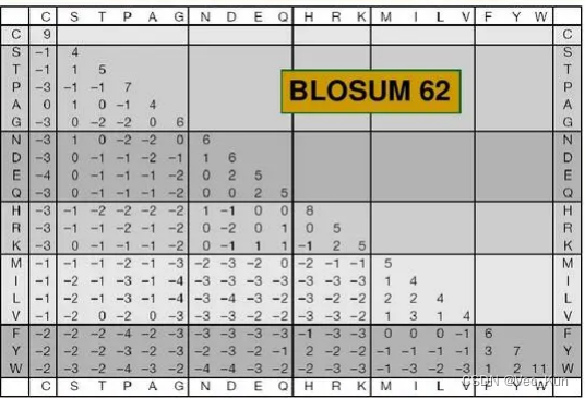
A. Using this matrix, two aligned cysteines (C) would receive a score of 9 while two aligned threonines (T) would only receive a score of 5. What can you conclude about cysteine relative to threonine?

Cysteines (C) is rarer than threonines (T) . The higher the match score the rarer the match.

B. A serine (S) aligned with a cysteine (C) would receive a negative score (-1) while a serine aligned with a threonine would receive a positive score (1). Offer a possible explanation for this in terms of physicochemical properties of the amino acid side chains.

The Mercapto is difficult to generate hydrogen bond than Hydroxyl

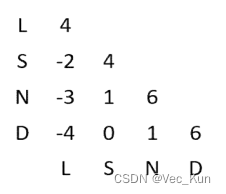
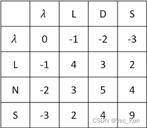
C. The bestng an alignment score. Use the BLOSUM62 matrix alignment of the two amino acid sequences “LDS” and “LNS” is obvious (it’s shown below). Given a scoring system, you could easily calculate an alignment score. Set up a matrix and use the dynamic programming algorithm to “prove” that this is the best alignment by calculating x (see Powerpoint notes) to score aligned residues, and use a gap penalty of -1. (You may hand write the matrix in your homework rather than typing it if you like.

It receives an alignment score of 4 + 1 + 4 = 9

The matrix verifies this is the maximum possible alignment score using these sequences and rules. So it proves this alignment is optimal.

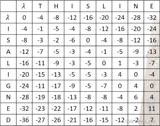
3. Find the optimal global alignment of the two sequences Seq1: THISLINE and Seq2: ISALIGNED based on the BLOSUM62 matrix with linear gap penalty of -4.

Multiple sequence alignment

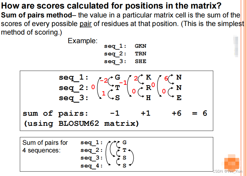
*全动态编程对于多序列比对是不实用的。序列长残基多时候比较指数增长

* Categories of Heuristic Algorithms for Multiple Sequence Alignment:

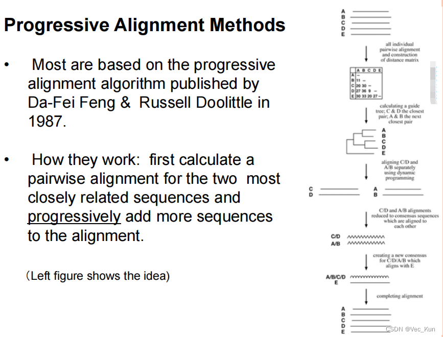
1. Progressive alignment methods

【first calculate a pairwise alignment for the two most closely related sequences and

progressively add more sequences to the alignment.】P8/p16

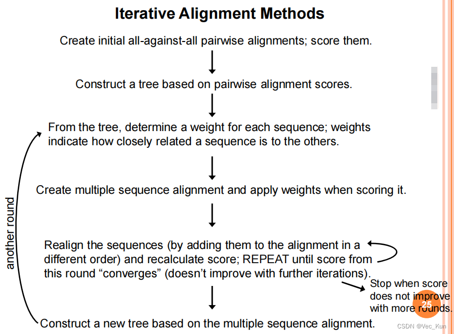
2. Iterative alignment methods

【Iterative alignment methods attempt to correct a problem of progressive methods:

Errors in the initial alignments of the most closely related sequences are propagated to the final multiple sequence alignment.】

PSSM方法

【PSSM中的每个值是在多序列比对中给定位置处观察到的该氨基酸的计数除以在比对中该位置处该氨基酸的预期计数的比率。然后将该值转换为对数刻度（通常以2为基数）。

PSSM中的值反映了任何给定氨基酸出现在比对中的每个位置的概率，以及在比对中每个位置的保守或非保守取代的影响。】

Motifs and domains

*Motif– a short conserved sequence pattern; can be just a few amino acid residues, up to ~20.

*Domain– a longer conserved sequence pattern which adopts a particular three-dimensional structure and is an independent functional and structural unit; typically 40-700 residues.

*吉布斯采样算法吉布斯采样是一个原理上类似于EM的迭代过程，但算法不同。在每次迭

代中，移除一个序列，并从剩余序列中构建试验比对。与EM一样，Gibbs采样在一组序

列中搜索统计上最可能的基序，并可以在每个序列中找到这些基序的最佳宽度和数量。

*配置文件HMM：轮廓HMM可以从一组未对齐的序列中构建。对模型的长度（匹配状态的数量）和概率参数进行了初步猜测。然后通过迭代更新概率参数来训练模型（该过程可以使用各种算法）。

* EM-algorithm：Step 1. Maximization Step 2. Expectation Step 3. Repeat Step 1 and 2.

期望最大化(Expectation Maximization, EM)算法该算法通过迭代的方法从一组序列中发现统计上最可能的基序模式(motif或domain)。它不依赖于事先产生的多重序列比对。
吉布斯采样(Gibbs Sampler)算法
与EM算法类似的迭代过程,也能在一组序列中发现motif或domain,并能找出每条序列中这些模式的最佳长度和数量。
配置隐马尔可夫模型(Profile Hidden Markov Model) 可以从一组未比对的序列中构建。通过迭代更新概率参数对模型进行训练。

这些都是用统计学方法从序列数据集中学习motif和domain的无监督学习算法。不需要事先的序列比对就能发现序列模式。

Homework 4

Identifying protein motifs using Expectation Maximization (EM) algorithm.

Suppose we have 200 protein sequences of length 100, in the dataset. Each character represents an amino acid. The length of the motif is 10. The figure below shows the first 10 samples in the dataset.

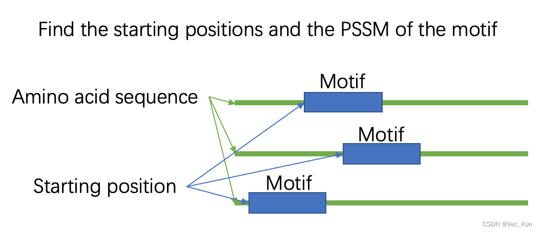Write a program to identify the starting position of the motif in each protein sequence. Write a report which includes: a) your understanding on EM algorithm, b) the core algorithm, c) the final result (starting positions and PSSM of the motif), d) the difficulties you met.

My understanding to Expectation Maximization(EM) Algorithm:

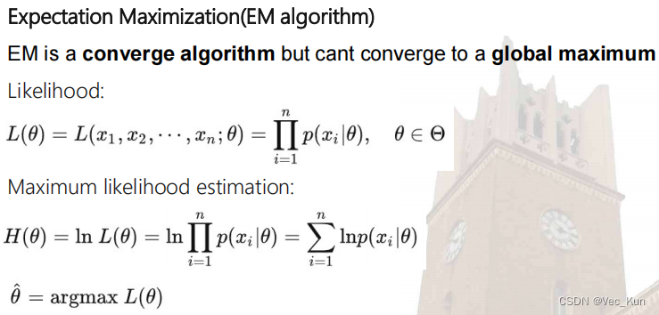
The EM algorithm is an iterative method that estimates model parameters where there are missing, hidden, or unobserved values.
It proceeds in two steps that are repeated until convergence:
1. Expectation (E) Step: Creating a function for the expectation of the log-likelihood evaluated using the current estimate for parameters. This involves estimating values for latent variables based on the current parameter values.
2. Maximization (M) Step: Finding parameters that maximize the expected log-likelihood found on the E step. These become the new parameter estimates.
By iteratively doing E and M steps, EM finds the parameters that locally maximize the likelihood of the data comprising both observed and unobserved values.
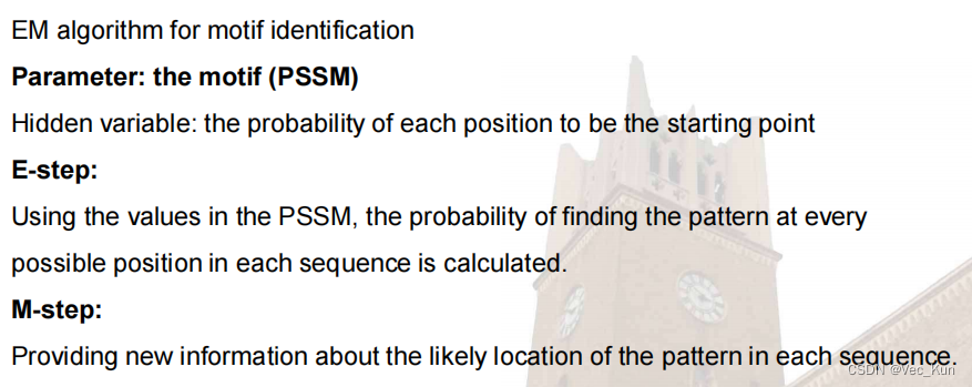
For motif finding, the "unobserved" data are the true starting positions of each motif instance. The expectation step estimates motif locations, while the maximization step finds an updated motif model that fits best based on those expected motif positions.

Core Algorithm:

Fake code:

Initialize motif starting positions randomly in each sequence
E-step:
1. Extract motif instances from each sequence based on current start positions
2. Calculate probability of each position being the true start given current motif model
M-step:
1. Update start position for each sequence to position with highest probability from E-step
2. Update PSSM for motif based on new aligned motif instances
Repeat E-step and M-step until convergence
Output final motif start positions and PSSM

Code in PyCharm: (python=3.8)

# Created at WASEDA Univ.
# Author: Vector Kun
# Time: 2023/12/17 12:44import csv
from random import randint as randint
from math import log as log
import matplotlib.pyplot as plt
from numpy import mean
from matplotlib.pyplot import MultipleLocator# Define basic parameters
proteinsDataset = "proteins.csv"
resultFile = "result.txt"
trainNum = 200
trainTime = 10
motif_length = 10def csv_reader(path):"""Read data from csv"""origin_protein_list = []with open(path) as f:reader = csv.reader(f)for item in reader:origin_protein_list.append(item)# print(origin_protein_list)return origin_protein_listdef data_preprocess(path):"""Remove order in the data"""protein_order_list = csv_reader(path)[1:]protein_list = []for protein in protein_order_list:protein_list.append(protein[1:])# print(protein_list)return protein_listdef matrix_transposition(matrix):"""Transpose the matrix"""new_matrix = []for i in range(len(matrix[0])):matrix1 = []for j in range(len(matrix)):matrix1.append(matrix[j][i])new_matrix.append(matrix1)# print(new_matrix)return new_matrixdef PSSM_calculation(seqs):"""Calculate pssm matrix"""# The species of the aminosamino_acids_list = ['A', 'C', 'D', 'E', 'F','G', 'H', 'I', 'K', 'L','M', 'N', 'P', 'Q', 'R','S', 'T', 'V', 'W', 'Y']# PSSM matrixweight_matrix = {}# Frequency of amino acidsfre_matrix = {}# Number of occurrences of amino acids at each positioncount_matrix = {}# Initializationfor amino in amino_acids_list:count_matrix[amino] = [0] * motif_lengthfre_matrix[amino] = 0weight_matrix[amino] = [0] * motif_length# Calculate the number of amino acids in each positioncol_num = 0new_seqs = matrix_transposition(seqs)for col in new_seqs:for amino in col:i = col_numcount_matrix[amino][i] += 1col_num += 1# Calculate the frequency of amino acidsfor amino in count_matrix:amino_sum = 0for count in count_matrix[amino]:amino_sum += countfrequency = amino_sum / (len(seqs) * motif_length)fre_matrix[amino] = frequency# Calculate weight matrixfor i in range(0, motif_length):for amino in count_matrix:# Calculate WM by dividing it by the total nums of swqscount_divided_nums = count_matrix[amino][i] / len(seqs)if fre_matrix[amino] == 0:weight = 0# Calculate WM by dividing it by the frequency of the aminoselse:weight = count_divided_nums / fre_matrix[amino]# Logarithmic operation on matrixif weight == 0:weight = -10else:weight = log(weight, 10)weight_matrix[amino][i] += float(format(weight, '.4f'))# print(count_matrix, '\n', fre_matrix, '\n', weight_matrix, '\n')return weight_matrixdef get_random_seqs(protein_list):"""Randomly initialize the starting position"""train_seq = []for i in range(0, trainNum):head = randint(0, 90)tail = head + motif_lengthseq = protein_list[i][head:tail]train_seq.append(seq)# print(train_seq)return train_seqdef cal_score(seqs, weight_matrix):"""Calculate the score based on sequences and the WM"""score = 0for i in range(0, motif_length):score += weight_matrix[seqs[i]][i]return scoredef get_train_seqs(protein_list, weight_matrix):"""Calculate scores os all the motifs with different starting position, select the optimal position """max_score = []train_seqs = []max_index = []for protein in protein_list:score_list = []for i in range(0, 90):test_seq = protein[i:i + motif_length]# Calculate scores of different position in one proteinscore_list.append(cal_score(test_seq, weight_matrix))# Get the max onemax_position = score_list.index(max(score_list))# Get the optimal sequences of one proteinnew_train_seq = protein[max_position:max_position + motif_length]# Get the best score to cal avemax_score.append(max(score_list))train_seqs.append(new_train_seq)max_index.append(max_position)return train_seqs, max_index, max_scoredef data_training(protein_list):"""Train the data"""# Number of iterationsiteration_num = 100Best_ave = 0Best_iteration = 0for i in range(iteration_num):# Average score of every iterationmax_score_list = []# Initialize the position randomly firsttrain_seq = get_random_seqs(protein_list)# Calculate PSSM matrixweight_matrix = PSSM_calculation(train_seq)for j in range(0, iteration_num):# Estimate and choose the best positionnew_train_seqs, max_index, max_score = get_train_seqs(protein_list, weight_matrix)# Calculate new matrixweight_matrix = PSSM_calculation(new_train_seqs)max_score_list.append(mean(max_score))# Plot convergencegeneration = []for k in range(1, iteration_num + 1):generation.append(k)max_score_list = []plt.plot(generation, max_score_list)y_major_locator = MultipleLocator(0.3)ax = plt.gca()ax.yaxis.set_major_locator(y_major_locator)plt.ylabel('Mean scores', fontsize=10)plt.show()# Write the result to txtf = open("result.txt", "a")f.write("\n" + f"Iteration {i}" + '\n' + "Starting positions:" + str(max_index))f.write('\n' + "PSSM:" + str(weight_matrix))f.write('\n' + "Scores:" + str(max_score_list))f.write('\n' + "Average best score:" + str(mean(max_score)))# Get the max scoreif Best_ave <= mean(max_score):Best_ave = mean(max_score)Best_iteration = iprint(f"Iteration {i}: Best average score = {Best_ave}")print('Best iteration: ', Best_iteration)if __name__ == '__main__':fl = open("result.txt", "wt")fl.close()# Get the protein listproteinList = data_preprocess(proteinsDataset)data_training(proteinList)

The final result:

D:\Anaconda3\envs\spider\python.exe 
Iteration 0: Best average score = 4.3729255
Best iteration:  0
Iteration 1: Best average score = 5.199039
Best iteration:  1
Iteration 2: Best average score = 5.199039
Best iteration:  1
Iteration 3: Best average score = 5.199039
Best iteration:  1
Iteration 4: Best average score = 6.680054999999999
Best iteration:  4
Iteration 5: Best average score = 6.680054999999999
Best iteration:  4
Iteration 6: Best average score = 6.680054999999999
Best iteration:  4
Iteration 7: Best average score = 6.680054999999999
Best iteration:  4
Iteration 8: Best average score = 6.680054999999999
Best iteration:  4
Iteration 9: Best average score = 6.680054999999999
Best iteration:  4
Iteration 10: Best average score = 6.680054999999999
Best iteration:  4
Iteration 11: Best average score = 6.680054999999999
Best iteration:  4
Iteration 12: Best average score = 6.680054999999999
Best iteration:  4
Iteration 13: Best average score = 6.680054999999999
Best iteration:  4
Iteration 14: Best average score = 6.680054999999999
Best iteration:  4
Iteration 15: Best average score = 6.680054999999999
Best iteration:  4
Iteration 16: Best average score = 6.680054999999999
Best iteration:  4
Iteration 17: Best average score = 6.680054999999999
Best iteration:  4
Iteration 18: Best average score = 6.680054999999999
Best iteration:  4
Iteration 19: Best average score = 6.680054999999999
Best iteration:  4
Iteration 20: Best average score = 6.680054999999999
Best iteration:  4
Iteration 21: Best average score = 6.680054999999999
Best iteration:  4
Iteration 22: Best average score = 6.680054999999999
Best iteration:  4
Iteration 23: Best average score = 6.680054999999999
Best iteration:  4
Iteration 24: Best average score = 6.680054999999999
Best iteration:  4
Iteration 25: Best average score = 6.680054999999999
Best iteration:  4
Iteration 26: Best average score = 6.680054999999999
Best iteration:  4
Iteration 27: Best average score = 6.680054999999999
Best iteration:  4
Iteration 28: Best average score = 6.680054999999999
Best iteration:  4
Iteration 29: Best average score = 6.680054999999999
Best iteration:  4
Iteration 30: Best average score = 6.680054999999999
Best iteration:  4
Iteration 31: Best average score = 6.680054999999999
Best iteration:  4
Iteration 32: Best average score = 6.832890500000001
Best iteration:  32
Iteration 33: Best average score = 6.832890500000001
Best iteration:  32
Iteration 34: Best average score = 6.832890500000001
Best iteration:  32
Iteration 35: Best average score = 6.832890500000001
Best iteration:  32
Iteration 36: Best average score = 6.832890500000001
Best iteration:  32
Iteration 37: Best average score = 6.855327999999999
Best iteration:  37
Iteration 38: Best average score = 6.870583999999999
Best iteration:  38
Iteration 39: Best average score = 6.870583999999999
Best iteration:  38
Iteration 40: Best average score = 6.9964825
Best iteration:  40
Iteration 41: Best average score = 6.9964825
Best iteration:  40
Iteration 42: Best average score = 7.2110034999999995
Best iteration:  42
Iteration 43: Best average score = 7.2110034999999995
Best iteration:  42
Iteration 44: Best average score = 7.2110034999999995
Best iteration:  42
Iteration 45: Best average score = 7.2110034999999995
Best iteration:  42
Iteration 46: Best average score = 7.2110034999999995
Best iteration:  42
Iteration 47: Best average score = 7.2110034999999995
Best iteration:  42
Iteration 48: Best average score = 7.2110034999999995
Best iteration:  42
Iteration 49: Best average score = 7.2110034999999995
Best iteration:  42
Iteration 50: Best average score = 7.2110034999999995
Best iteration:  42
Iteration 51: Best average score = 7.2110034999999995
Best iteration:  42
Iteration 52: Best average score = 7.2110034999999995
Best iteration:  42
Iteration 53: Best average score = 7.2110034999999995
Best iteration:  42
Iteration 54: Best average score = 7.2110034999999995
Best iteration:  42
Iteration 55: Best average score = 7.2110034999999995
Best iteration:  42
Iteration 56: Best average score = 7.2110034999999995
Best iteration:  42
Iteration 57: Best average score = 7.2110034999999995
Best iteration:  42
Iteration 58: Best average score = 7.2110034999999995
Best iteration:  42
Iteration 59: Best average score = 7.2110034999999995
Best iteration:  42
Iteration 60: Best average score = 7.2110034999999995
Best iteration:  42
Iteration 61: Best average score = 7.2110034999999995
Best iteration:  42
Iteration 62: Best average score = 7.2110034999999995
Best iteration:  42
Iteration 63: Best average score = 7.2110034999999995
Best iteration:  42
Iteration 64: Best average score = 7.2110034999999995
Best iteration:  42
Iteration 65: Best average score = 7.2110034999999995
Best iteration:  42
Iteration 66: Best average score = 7.2110034999999995
Best iteration:  42
Iteration 67: Best average score = 7.2110034999999995
Best iteration:  42
Iteration 68: Best average score = 7.2110034999999995
Best iteration:  42
Iteration 69: Best average score = 7.2110034999999995
Best iteration:  42
Iteration 70: Best average score = 7.2110034999999995
Best iteration:  42
Iteration 71: Best average score = 7.2110034999999995
Best iteration:  42
Iteration 72: Best average score = 7.2110034999999995
Best iteration:  42
Iteration 73: Best average score = 7.2110034999999995
Best iteration:  42
Iteration 74: Best average score = 7.2110034999999995
Best iteration:  42
Iteration 75: Best average score = 7.2110034999999995
Best iteration:  42
Iteration 76: Best average score = 7.2110034999999995
Best iteration:  42
Iteration 77: Best average score = 7.2110034999999995
Best iteration:  42
Iteration 78: Best average score = 7.2110034999999995
Best iteration:  42
Iteration 79: Best average score = 7.2110034999999995
Best iteration:  42
Iteration 80: Best average score = 7.2110034999999995
Best iteration:  42
Iteration 81: Best average score = 7.2110034999999995
Best iteration:  42
Iteration 82: Best average score = 7.2110034999999995
Best iteration:  42
Iteration 83: Best average score = 7.2110034999999995
Best iteration:  42
Iteration 84: Best average score = 7.2110034999999995
Best iteration:  42
Iteration 85: Best average score = 7.2110034999999995
Best iteration:  42
Iteration 86: Best average score = 7.2110034999999995
Best iteration:  42
Iteration 87: Best average score = 7.2110034999999995
Best iteration:  42
Iteration 88: Best average score = 7.2110034999999995
Best iteration:  42
Iteration 89: Best average score = 7.2110034999999995
Best iteration:  42
Iteration 90: Best average score = 7.2110034999999995
Best iteration:  42
Iteration 91: Best average score = 7.2110034999999995
Best iteration:  42
Iteration 92: Best average score = 7.2110034999999995
Best iteration:  42
Iteration 93: Best average score = 7.2110034999999995
Best iteration:  42
Iteration 94: Best average score = 7.2110034999999995
Best iteration:  42
Iteration 95: Best average score = 7.2110034999999995
Best iteration:  42
Iteration 96: Best average score = 7.2110034999999995
Best iteration:  42
Iteration 97: Best average score = 7.2110034999999995
Best iteration:  42
Iteration 98: Best average score = 7.2110034999999995
Best iteration:  42
Iteration 99: Best average score = 7.2110034999999995
Best iteration:  42Process finished with exit code 0

From the output, we can get:

Iteration 99: Best average score = 7.2110034999999995
Best iteration: 42

So the best average score of 100 iterations is roughly 7.211, which iteration number is 42.

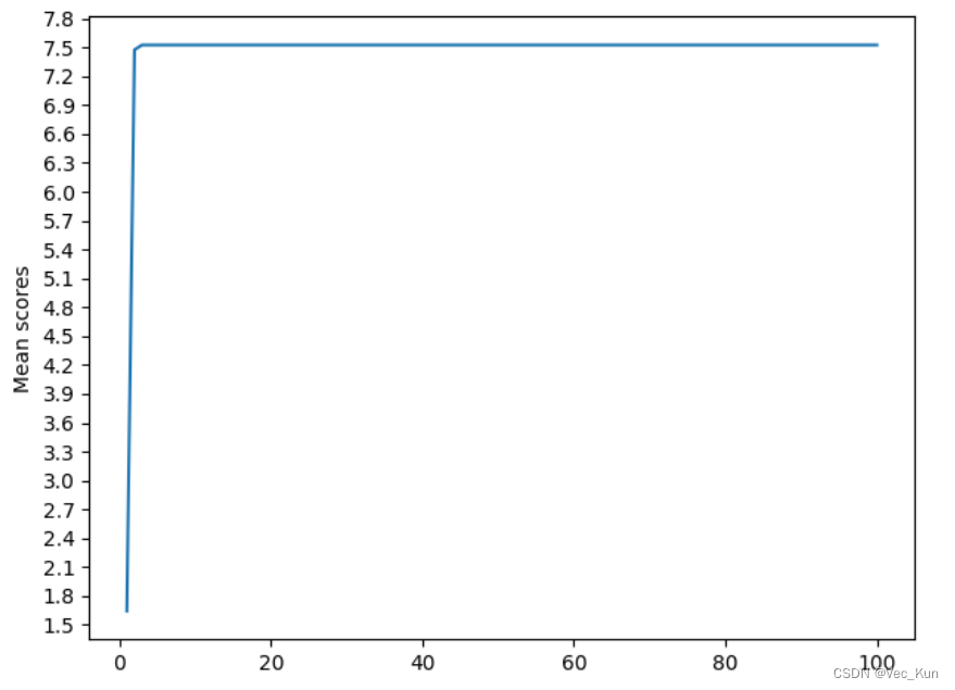
The Convergence Plot is shown below:

The result to iteration 42 in result.txt is:

Iteration 42
Starting positions:[40, 23, 0, 57, 8, 73, 49, 85, 29, 46, 82, 4, 49, 14, 32, 23, 78, 41, 0, 43, 69, 82, 76, 3, 25, 5, 36, 82, 34, 74, 30, 89, 15, 54, 42, 49, 84, 66, 71, 22, 23, 11, 51, 31, 77, 45, 30, 83, 48, 7, 80, 45, 60, 33, 84, 82, 86, 13, 79, 22, 21, 12, 68, 69, 81, 38, 68, 64, 89, 65, 47, 58, 53, 12, 56, 30, 12, 72, 16, 85, 57, 42, 86, 81, 30, 8, 6, 65, 32, 82, 24, 53, 11, 26, 15, 75, 44, 41, 56, 7, 27, 76, 34, 63, 46, 9, 32, 35, 13, 27, 88, 78, 86, 76, 26, 26, 74, 44, 51, 74, 29, 87, 46, 8, 64, 34, 13, 5, 57, 19, 80, 10, 68, 1, 28, 23, 33, 34, 56, 88, 63, 41, 57, 31, 30, 29, 8, 51, 26, 29, 31, 58, 69, 84, 47, 1, 55, 88, 34, 55, 65, 66, 7, 7, 89, 76, 60, 58, 37, 73, 84, 87, 24, 6, 18, 14, 83, 1, 60, 16, 68, 42, 31, 10, 47, 8, 57, 32, 52, 51, 32, 59, 64, 2, 72, 26, 66, 58, 7, 5]
PSSM:{'A': [0.9723, -1.2504, -0.9494, -1.2504, -10.0, -1.2504, -0.6484, -0.9494, -10.0, -10.0], 'C': [-1.5514, -1.5514, 0.6891, -1.2504, -1.5514, -10.0, -1.2504, 0.6841, -1.2504, -1.5514], 'D': [-0.0414, -0.3424, -0.3424, -10.0, 0.1347, 0.1347, 0.1347, -0.0414, 0.3565, -0.0414], 'E': [-0.0414, 0.2596, -0.0414, -10.0, -0.0414, -0.0414, -10.0, -10.0, 0.2596, 0.4357], 'F': [0.1549, 0.331, 0.5528, -10.0, -10.0, -0.1461, -0.1461, -10.0, 0.1549, -10.0], 'G': [-0.9661, -0.6651, -0.7901, -0.9661, -10.0, -1.2672, -10.0, -0.9661, 0.9658, -10.0], 'H': [-10.0, 0.0706, 0.2467, 0.2467, -10.0, -10.0, -0.2304, 0.3716, 0.0706, 0.0706], 'I': [-10.0, -10.0, 0.301, -10.0, 0.426, -10.0, -0.1761, 0.301, 0.1249, 0.1249], 'K': [-0.1761, 0.426, -10.0, -0.1761, 0.426, -0.1761, -0.1761, -10.0, 0.1249, -0.1761], 'L': [-1.2648, -1.2648, -1.2648, -1.2648, -10.0, 0.9807, -0.7877, -1.2648, -10.0, -10.0], 'M': [-10.0, -0.0792, -10.0, 0.6198, 0.2218, -10.0, 0.2218, -10.0, -0.0792, -0.0792], 'N': [0.5229, -10.0, -10.0, -0.0792, -10.0, -0.0792, -10.0, -0.0792, -0.0792, 0.5229], 'P': [-10.0, -10.0, -1.2492, 0.6977, -10.0, -1.5502, -1.5502, -10.0, -1.5502, 0.6878], 'Q': [0.301, -10.0, -0.1761, -10.0, -0.1761, 0.301, -0.1761, 0.1249, 0.1249, 0.1249], 'R': [-0.0212, 0.1549, -10.0, 0.2798, -0.3222, -0.0212, 0.4559, -0.0212, -10.0, -0.3222], 'S': [-0.7924, 0.9685, -10.0, -1.2695, -10.0, -0.9685, -0.7924, -0.6675, -10.0, -10.0], 'T': [-1.2553, -1.2553, -1.2553, -10.0, -0.9542, -10.0, 0.9726, -10.0, -0.9542, -0.6532], 'V': [-0.9845, -0.9845, -10.0, -1.2856, 0.9721, -0.9845, -0.9845, -1.2856, -0.9845, -10.0], 'W': [0.426, -0.1761, 0.301, -10.0, -10.0, 0.1249, -10.0, -0.1761, 0.301, -0.1761], 'Y': [0.4559, -10.0, -10.0, -0.1461, -10.0, 0.331, -10.0, 0.331, -10.0, 0.331]}
Scores:[1.6438155, 7.475081, 7.525479999999999, 7.525479999999999, 7.525479999999999, 7.525479999999999, 7.525479999999999, 7.525479999999999, 7.525479999999999, 7.525479999999999, 7.525479999999999, 7.525479999999999, 7.525479999999999, 7.525479999999999, 7.525479999999999, 7.525479999999999, 7.525479999999999, 7.525479999999999, 7.525479999999999, 7.525479999999999, 7.525479999999999, 7.525479999999999, 7.525479999999999, 7.525479999999999, 7.525479999999999, 7.525479999999999, 7.525479999999999, 7.525479999999999, 7.525479999999999, 7.525479999999999, 7.525479999999999, 7.525479999999999, 7.525479999999999, 7.525479999999999, 7.525479999999999, 7.525479999999999, 7.525479999999999, 7.525479999999999, 7.525479999999999, 7.525479999999999, 7.525479999999999, 7.525479999999999, 7.525479999999999, 7.525479999999999, 7.525479999999999, 7.525479999999999, 7.525479999999999, 7.525479999999999, 7.525479999999999, 7.525479999999999, 7.525479999999999, 7.525479999999999, 7.525479999999999, 7.525479999999999, 7.525479999999999, 7.525479999999999, 7.525479999999999, 7.525479999999999, 7.525479999999999, 7.525479999999999, 7.525479999999999, 7.525479999999999, 7.525479999999999, 7.525479999999999, 7.525479999999999, 7.525479999999999, 7.525479999999999, 7.525479999999999, 7.525479999999999, 7.525479999999999, 7.525479999999999, 7.525479999999999, 7.525479999999999, 7.525479999999999, 7.525479999999999, 7.525479999999999, 7.525479999999999, 7.525479999999999, 7.525479999999999, 7.525479999999999, 7.525479999999999, 7.525479999999999, 7.525479999999999, 7.525479999999999, 7.525479999999999, 7.525479999999999, 7.525479999999999, 7.525479999999999, 7.525479999999999, 7.525479999999999, 7.525479999999999, 7.525479999999999, 7.525479999999999, 7.525479999999999, 7.525479999999999, 7.525479999999999, 7.525479999999999, 7.525479999999999, 7.525479999999999, 7.525479999999999]
Average best score:7.2110034999999995

The difficulties I met:

Determining suitable stopping criteria and determining when the algorithm has converged to a stable solution. In practice, heuristics like a maximum number of iterations are used.
Avoid getting stuck in poor local optima rather than the global optimum. Using multiple random restarts can mitigate this issue.
Runtime complexity for large datasets. Matrix computations may be intensive for large sequence sets and long motifs. Parallelization and approximation methods can improve scalability.
Interpreting the resulting motif model. Statistical significance testing should be done to evaluate if the identified motif represents a true common signal vs random shared patterns.

Machine Learning Approaches

GA for sequencing and MSA

Sequencing by Using GA

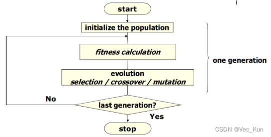
GA – Genetic Algorithm（基因互换、变异）

EDA – Estimation of Distribution Algorithm

*Sequencing by Using GA

Multiple Sequence Alignments Using GA

*Using Genetic Algorithms for Pairwise and Multiple Sequence Alignments

Protein Function Prediction

Gene Function Prediction Using SVM

本节讨论了使用SVM进行基因功能预测的多标签分类和层次多标签分类方法。

主要内容有:

1. 基于标签排序和精细决策边界SVM的多标签分类方法。该方法考虑了样本重叠的信息,通过Bias模型改进重叠样本的分类准确率;并提出了一个基于输入实例和标签排序的实例相关阈值选取策略。

2. 基于过采样和层次约束的层次多标签分类方法。该方法通过提出分层SMOTE方法解决数据集不平衡问题;并通过在TPR规则集成中引入分类器性能权重来改进集成,限制差分类器的错误传播效应。

3. 在Yeast和Genbase数据集上的试验表明,上述两种方法在基因功能预测任务上都能取得不错的性能。

4. 这些方法为解决基因测序数据的功能标注与分类问题提供了有效的机器学习框架。

Protein Function Prediction Using DNN

本节主要内容是关于使用深度迁移学习方法进行蛋白质功能预测的研究。

主要有以下几个方面:

1. 使用多头多尾深度卷积神经网络模型进行基因本体论(GO)注释预测。该模型可以实现知识迁移,提高模型性能。

2. 通过GO注释预测的迁移学习来增强亚细胞定位预测。共享特征提取器,实现预训练和微调。

3. 基于迁移学习的蛋白质相互作用预测,用于复合物检测。迁移模型从GO和定位注释任务中学习知识。

4. 在GO注释、定位和相互作用预测任务之间实现了迁移学习。提出的模型可以扩展到其他生物信息学任务。

5. 试验结果表明,迁移学习可以有效改进蛋白质功能预测的性能。

总体而言,本节研究了如何利用深度学习和迁移学习的方法,改进蛋白质功能预测与标注的性能。

Protein Structure Prediction

Protein Folding Based on EDA

本节主要内容是关于使用基于EDA的混合智能算法进行蛋白质结构预测的研究。

主要包含以下几个方面:

1. 使用混合EDA算法求解简化的HP模型蛋白质折叠问题。提出复合适应度函数、引导算子局部搜索和改进的回溯修复方法。

2. 提出自适应分群EDA算法,使用亲和传播聚类实现自适应分群,并使用玻尔兹曼机制实现平衡搜索。应用于连续优化和HP模型蛋白质结构预测问题。

3. 试验结果表明,所提出的混合EDA和自适应分群EDA算法都可以有效提高蛋白质结构预测的性能。

4. EDA算法与特定问题信息的结合为解决蛋白质结构预测等复杂优化问题提供了一种有效途径。

总的来说, 它探讨了EDA算法在蛋白质结构预测问题上的应用,以及如何设计出性能更优的混合EDA和自适应EDA算法。

Protein Folding Based on Deep Reinforcement Learning

本节是关于蛋白质折叠问题的研究报告。主要内容包括:

1. 简介蛋白质折叠问题和HP模型
2. 深度强化学习方法用于解决HP模型中的蛋白质折叠问题
3. AlphaGo系列中蒙特卡洛树搜索(MCTS)的应用
4. 将MCTS应用于HP模型以解决蛋白质折叠问题
5. 蛋白质结构预测的最新进展,如AlphaFold

报告介绍了如何通过深度强化学习和蒙特卡洛树搜索等方法来预测蛋白质序列的三维结构,这是蛋白质折叠问题的核心。总的来说,这篇报告聚焦在利用AI技术来解决蛋白质结构预测这个基础科学难题上。

AlphaFold2 for Protein Structure Prediction

本节是关于AlphaFold2蛋白质结构预测方法的介绍和分析报告。主要内容包括:

1. 蛋白质折叠问题的背景简介
2. AlphaFold2的整体流程概览,包括数据准备、嵌入、Evoformer模块、结构模块等
3. AlphaFold2的具体技术细节,如多序列比对、表征提取、注意力机制、损失函数等
4. AlphaFold2预测蛋白质结构的应用,如蛋白质结构数据库

简而言之,这是一篇介绍和分析AlphaFold2在蛋白质结构预测领域里程碑式的进展的报告。它概述了这一最先进的AI系统是如何解决这一困扰生物学家50年之久的难题的。总的来说,这篇报告聚焦在利用深度学习技术来推动基础科学发展方面的内容。

References

EMBL-EBI, A Quick Introduction to Elements of Biology - Cells, Molecules, Genes, Functional Genomics, Microarrays
DOE Human Genome Program: Primer on Molecular Genetics, 1992
Jin Xiong, Essential Bioinformatics, Cambridge University Press, 2006
P. Larranaga et.al., "Machine Learning in Bioinformatics", Briefings in Bioinformatics, 7(1), 86-112, 2006
J.M. Claverie and C. Notredame, Bioinformatics for Dummies, 2nd Ed., Wiley Publishing Inc, 2007
B. Alberts et.al., Molecular Biology of THE CELL, 5th Ed., Garland Science, 2008
N.C. Jones and P.A. Pevzner, An Introduction to Bioinformatics Algorithms, The MIT Press, 2004
DNAFTB: DNA from the Beginning (An animated primer of 75 experiments that made modern genetics)