机器学习的要素
基本概念
- 泛化: The ability to predict accurately the target for new examples that differ from those used in the training set is known as generalization.
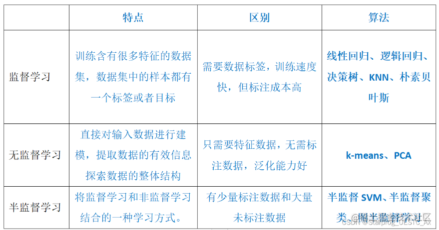
- 监督学习:The training data comprises examples of the input variable along with their corresponding target variable are known as supervised learning problems.
- 无监督学习:The training data consists of a set of inputs without any corresponding target value is called unsupervised learning problems.
- 回归:If the desired output is real-valued and continuous, is called regression.
- 分类:If the desired output consists of a finite number of discrete categories, then the task is called classification.
- 聚类:The goal is to discover groups of similar examples within the data, where is called clustering.
- 不确定性 Uncertainty in Machine Learning: (1)数据集里的噪点数据(Noise data in data set) (2)有限的数据集(Finite size of data sets)
Overfitting and underfitting
M 多项式

-
overfitting:Good performance on the training set, but poor performance on the testing set. The model is so complex that it captures noise or idiosyncratic features in the training data rather than generalizing to the true pattern of the overall data distribution.
-
如何解决 overfitting:
(1)正则化:One technique that is used to control the over-fitting phenomenon in such cases is that of regularisation, which involves adding a penalty term to the error function in order to discourage the coefficients from reaching large values.
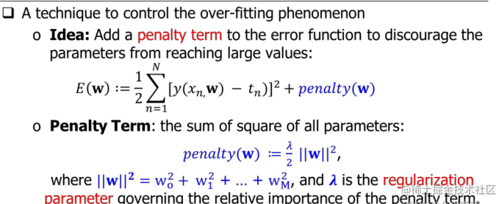
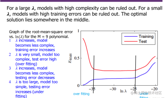
λ \lambda λ is a regularization parameter that we need to tune to determine its optimal value.
When the input is large, the penalty function penalty(w) will become large, then the first half of E(W) will become unimportant, the model will become simple, and both the training error and the test error will increase (underfitting occurs);
When the input is small, the model will become complex, the training error will be close to 0, and the performance will be excellent, while the test error will be close to 1, and the performance will be extremely poor (overfitting occurs at this point).
(2)Collect more training data
(3)Reduce the complexity of the model
(4)Use cross-validation to select appropriate model parameters and hyperparameters
(5)Dropout technique
-
underfitting: Poor performances on both training and valid (testing) datasets. The model is too simple to capture the underlying structure and relationships in the data.
-
如何解决 underfitting:
(1) Increase feature data to improve the degree of fitting and avoid under fitting.
(2) Increase the complexity of the model (increase the value of M) to improve the degree of fitting and avoid under fitting.
(3) Try to get more features
(4) Try adding polynomial features
(5) Try to reduce the degree of regularization
- overfitting and underfitting 和模型复杂度之间的关系
高偏差和低方差 = 欠拟合模型(低模型复杂度-M 小)
低偏差和高方差 = 过拟合模型(高度复杂的模型-M 大)
低偏差和低方差 = 最佳拟合模型(最佳模型)
➢ High bias and low variance = underfitting model (low model complexity-m small)
➢ Low bias and high variance = overfitting model (highly complex model-m large)
➢ Low bias and low variance = best fit model (best model)

- 泛化性能测量(Generalisation Performance)We obtain quantitative insight(定量洞察力) into the generalisation performance of a fitted model by **computing its error on the test set. **

均方误差(MSE): MSE = (1/n) * Σ(y_i - ŷ_i)^2 其中,n 表示样本数量,y_i 是第 i 个真实值,ŷ_i 是第 i 个预测值。
均方根误差(RMSE): RMSE = √MSE 即,RMSE 是 MSE 的平方根。
- Sigmoid Function

模型选择
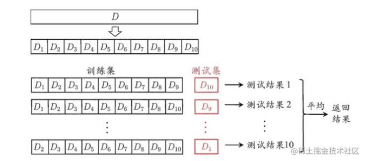
- K-Fold Cross-Validation:
-
将数据集随机打乱(Shuffle the dataset randomly).
-
将数据集随机分割为 k 组(randomly divide the data set into k groups).
-
对于每一个组,进行如下操作:(for each group, perform the following operations)
-
将这一个组的数据当做测试集(Take the data of this group as a test set)
-
剩余的 k−1 个组的数据当做训练集(The data of the remaining k-1 groups is used as the training set) ◼ 使用训练集训练模型,并在测试集上进行评测(Use the train set to train the model and evaluate it on the test set)
-
保留评测的分数,抛弃模型(Retain the evaluation score and discard the model)
-
-
使用 k 次评测分数的平均值来总结模型的性能。(Use the average value of K evaluation scores to summarize the performance of)
缺点(Drawback):
(1) The number of training runs that must be performed is increased by a factor of K, and this can prove problematic for models in which the training is itself computationally expensive.
(2) We might have multiple complexity parameters for a single model. Exploring combinations of settings for such parameters could, in the worst case, require a number of training runs that is exponential in the number of parameters, which is prohibitive
Leave-One-Out Cross Validation. It is a special case of K-Fold cross-validation where K is equal to the size of the training dataset. 留一法是 k 折交叉验证 k=m(m 为样本数)时候的特殊情况。即每次只留下一 个样本做测试集,其它样本做训练集,需要训练 k 次,测试 k 次。留一法计算 最繁琐,但样本利用率最高。因为计算开销较大,所以适合于小样本的情况。
- KNN
执行过程:
Step1: calculate the Euclidean distance between the new point and the existing point;
Step2: select the value of K and select the K neighbors nearest to the new point;
Step3: count the voting / prediction values of all k neighbors;
Step4: assign the new data point to the category with the largest number of neighbors.
K 取值较小时,模型复杂度高,训练误差会减小,泛化能力减弱,容易过拟合;K 取值较大时,模型复杂度低,训练误差会增大,泛化能力有一定的提高,但也容易欠拟合。When the value of K is small, the model complexity is high, the training error will be reduced, and the generalization ability will be weakened, may leads to overfitting; When the value of K is large, the model complexity is low, the training error will increase, and the generalization ability will be improved, may leads to underfitting.
原因 是 K 取值小的时候(如 k==1),仅用较小的领域中的训练样本进行预测,模型 拟合能力比较强,决策就是只要紧跟着最近的训练样本(邻居)的结果。但是,当训练集包含”噪声样本“时,模型也很容易受这些噪声样本的影响出现过拟合情况,噪声样本在哪个位置,决策边界就会画到哪,这样会增大"学习" 的方差,也就是容易过拟合。这时,多”听听其他邻居“训练样本的观点就能尽 量减少这些噪声的影响。 K 值取值太大时,情况相反,容易欠拟合。对于 K 值的选择,通常可以网格搜索,采用交叉验证的方法选取合适的 K 值
KNN 优缺点
优点:
➢ The algorithm is simple and intuitive, easy to apply to regression and multi classification tasks
➢ No hypothesis for data, high accuracy, less sensitive to out
➢ Since KNN method mainly depends on the surrounding finite adjacent samples, rather than the method of discriminating the class domain to determine the class, it is applicable to the cross or non-linear separable sample set of the class domain.
缺点:
➢ The calculation amount is large, especially when the sample size and feature number are very large.
➢ It is only related to a small number of k-adjacent samples. When the samples are unbalanced, the prediction accuracy of rare categories is low.
➢ The difference is small and it is not suitable for KNN integration to further improve performance
- KMeans
执行过程:
Step 1: randomly select k centroids (the value of K depends on how many classes you want to gather)
Step 2: calculate the distance between the sample and the center of mass. Those close to the center of mass are classified into one class and K classes
Step3: find the new centroid of each class after classification
Step4: calculate the distance from the sample to the new centroid again, and those close to the centroid are classified into one class Step5: judge whether the old and new clusters are the same. If they are the same, it means that the clustering has been successful. If not, cycle 2-4 steps until they are the same.
KMeans 优缺点
优点:
➢ The algorithm can prune the tree according to the category of fewer known clustering samples to determine the classification of some samples;
➢ In order to overcome the inaccuracy of clustering with a small number of samples, **the algorithm itself has the function of optimization iteration **
➢ The total clustering time complexity can be reduced because only a part of small samples are used.
缺点:
➢ It is necessary to determine an initial partition according to the initial clustering center, and then optimize the initial partition. The selection of this initial clustering center has a great impact on the clustering results. Once the initial value is not selected well, it may not be possible to obtain effective clustering results;
➢ The algorithm needs to continuously adjust the sample classification and calculate the new cluster center after adjustment. Therefore, when the data volume is very large, the time cost of the algorithm is very large
- Bootstrap-自助法(有放回重采样产生新数据)
执行流程
➢ 每次随机从 D 中挑选一个样本,将其拷贝放入D′,然后再将该样本放回初始数据集 D 中,使得该样本在下次采样时仍有可能被接收到;Each time, a sample is randomly selected from D, and it is copied into D, and then the sample is put back into the initial data set D, so that the sample may still be received in the next sampling;
➢ 这个过程重复执行 m 次后,我们就得到了包含 m 个样本的数据集 D′,这就 是自助采样的结果。After this process is repeated m times, we get the data set D 'containing m samples, which is the result of Bootstrap sampling.

Bootstrap 方法的优缺点
优点:
➢ The self-help method is very useful when the data set is small and it is difficult to effectively divide the training / test set;
➢ In addition, the self-help method can generate multiple different training sets from the initial data set, which is very beneficial to integrated learning and other methods
➢ Since we only need a small number of samples for bootstrapping, **the calculation requirements are very small **
缺点:
➢ The data set generated by bootstrap method changes the distribution of the initial data set, which will introduce estimation bias.
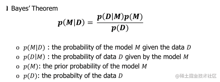
- 贝叶斯方法(Bayes)
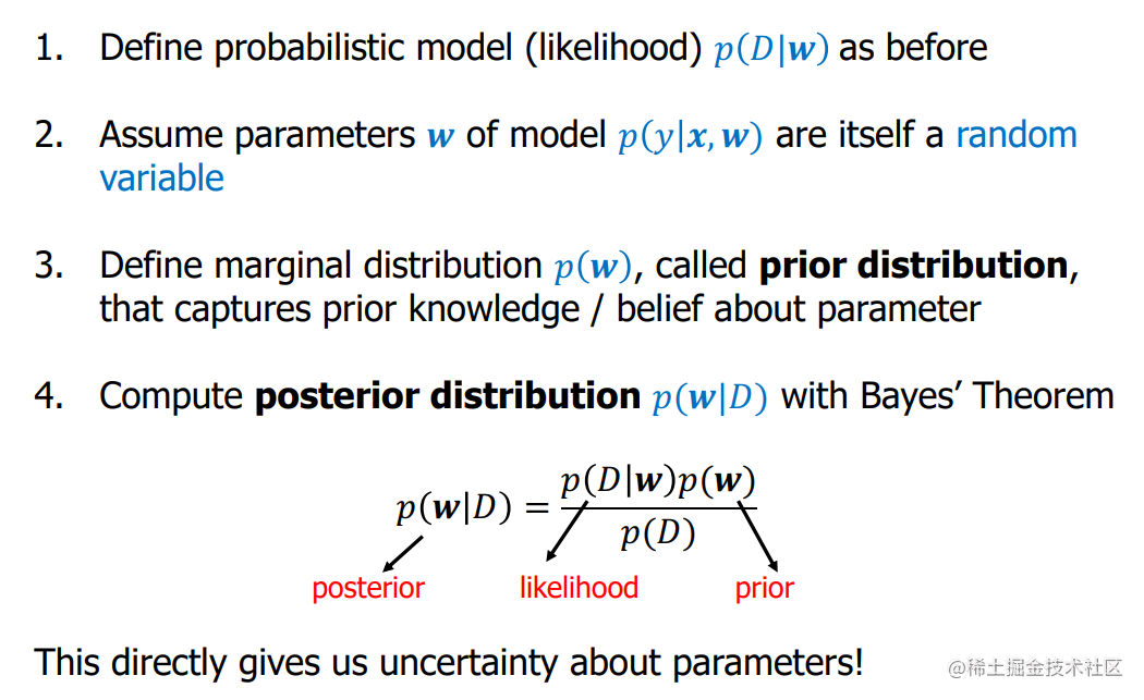
用贝叶斯方法对模型 w 进行估计的步骤:
- Continuous Random Variables 连续随机变量
We define the probability density function(pdf) for continuous random variables which must satisfy the following conditions:

An example of a famous probability density function for continuous random variables is the normal or Gaussian distribution.

其中 μ \mu μ 和 δ \delta δ 是分布的参数。可以证明, μ \mu μ是高斯分布的期望值(expectation), δ \delta δ是高斯分布的方差(variance)。
这个公式中的关键组成部分是指数项, 它导致了正态分布的特征钟形曲线。
- Maximum Likelihood Principle 最大似然原则
The maximum likelihood is a widely used parameter estimation technique in which the model parameters is set to the value that maximises the likelihood function p ( D ∣ m o d e l ) p(D\mid model) p(D∣model).
For a data point x n x_{n} xn from class C 1 C_{1} C1 , we have t n = 1 t_{n}=1 tn=1 hence

where N denotes the Gaussian distribution. Similarly for C 2 C_{2} C2 , we have t n = 0 t_{n}=0 tn=0 hence

Thus the likelihood function for all of the data points in the training set is:

As usual we work with the log-likelihood function since its optimisation is more convenient:

参数 µ 和 σ 的最大似然估计的关键思想是寻找参数值(choosing the value of parameters),使得在这些参数值下观察到数据的概率最大(the probability of the observed data set is maximised under these parameters),最大化似然函数 L(µ, σ) 以找到 µML 和 σML
偏导数=0的式子称之为封闭解
对于上面的正态分布来讲,其对应的最大似然函数应该是:
L ( μ , σ 2 ) = ∏ i = 1 N 1 2 π σ 2 e − ( x i − μ ) 2 2 σ 2 L(\mu, \sigma^2) = \prod_{i=1}^{N} \frac{1}{\sqrt{2\pi\sigma^2}} e^{-\frac{(x_i - \mu)^2}{2 \sigma^2}} L(μ,σ2)=∏i=1N2πσ21e−2σ2(xi−μ)2
为了简化计算,我们通常取对数似然函数(log-likelihood):
ln ( μ , σ 2 ) = ∑ i = 1 N [ − 1 2 ln ( 2 π σ 2 ) − ( x i − μ ) 2 2 σ 2 ] \ln(\mu, \sigma^2) = \sum_{i=1}^N [-\frac{1}{2}\ln(2\pi\sigma^2) - \frac{(x_i - \mu)^2}{2\sigma^2}] ln(μ,σ2)=∑i=1N[−21ln(2πσ2)−2σ2(xi−μ)2]
通过求解以下偏导数方程可以获得最大似然估计:
∂ ℓ ( μ , σ 2 ) ∂ μ = 0 ∂ ℓ ( μ , σ 2 ) ∂ ( σ 2 ) = 0 \frac{\partial \ell(\mu,\sigma^2)}{\partial \mu} = 0 \\ \frac{\partial \ell(\mu,\sigma^2)}{\partial (\sigma^2)} = 0 ∂μ∂ℓ(μ,σ2)=0∂(σ2)∂ℓ(μ,σ2)=0
Linear Regression 线性回归
Basis function


Squared Error and Maximum Likelihood
Loss function 损失函数
The objective of linear regression is to minimize the cost(error) function
The objective of the loss function is to optimize the weights of the model by minimizing this error


写下似然函数后,我们可以使用最大似然来确定参数,我们可以看到它是一个负对数似然关系。因此考虑关于W的最大化,这相当于最小化第二个项因为第一项相对于参数来说是常数,因此平方误差最小化是最大似然的最大化
After writing down the likelihood function, we can see that it is a negative log-likelihood relation. Therefore consider the maximization with respect to W, which is equivalent to minimizing the second term since the first term is constant with respect to the parameters, and therefore the squared error minimization is the maximization of the maximum likelihood

寻找最佳权重


Summary
-
Fitting criteria: find weights that minimise sum of squared errors 拟合标准:找到最小化平方误差之和的权重
-
How to identify minimum: derivative criterion 如何确定最小值:导数标准
-
For linear model with squared error: partial derivative ! is dot product of feature column ! with residual vector 对于有平方误差的线性模型:偏导数!是特征列的点积!与残差向量。
-
Derivative criterion: system of linear equations (normal equations) 导数准则:线性方程组(正常方程)。
-
Can be solved by linear algebra algorithm (elimination or iterative) 可以通过线性代数算法(消除法或迭代法)来解决。
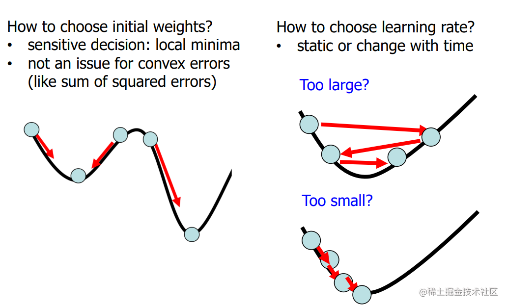
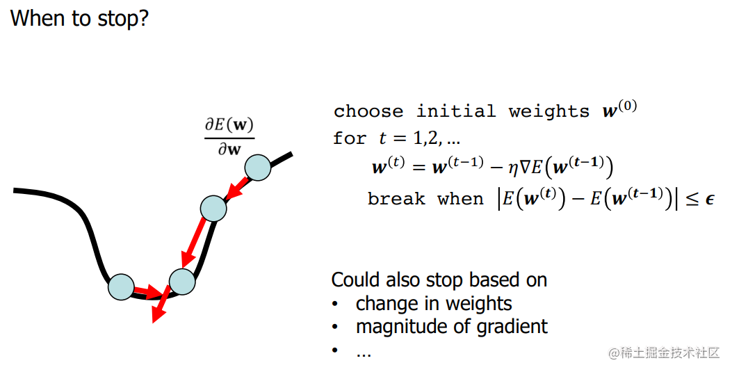
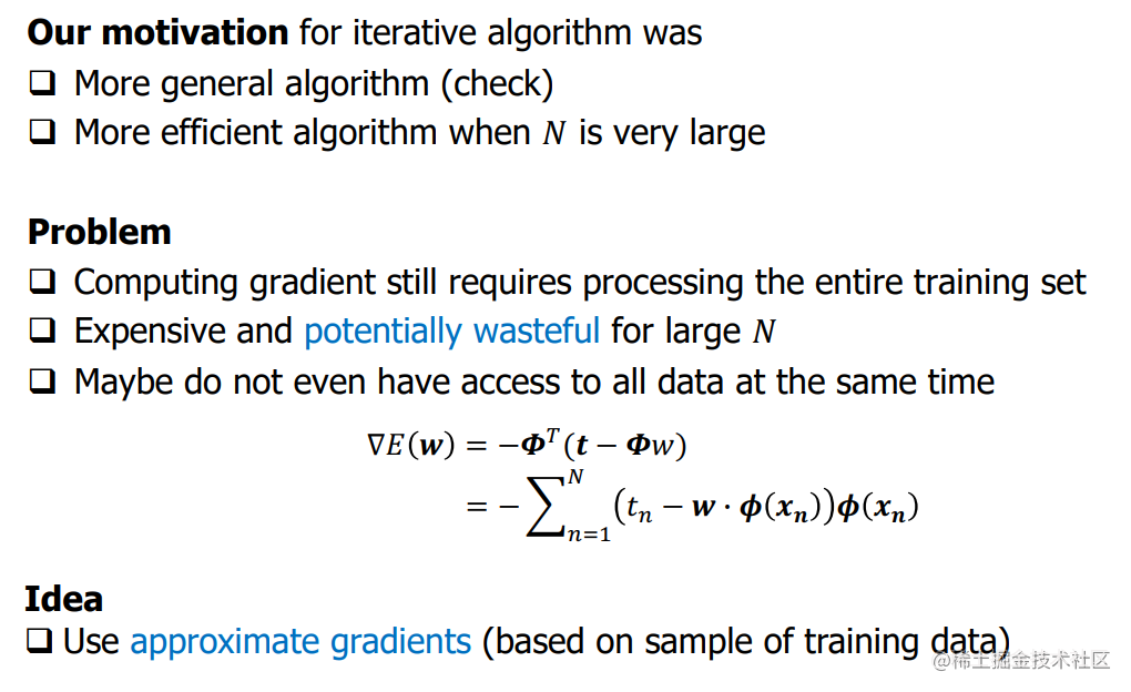
Gradient Descent Algorithm (GD)
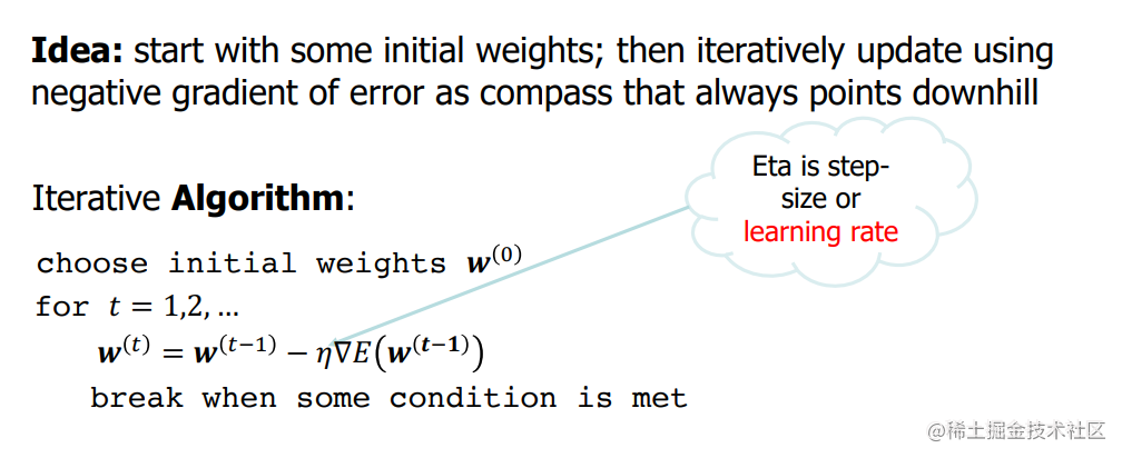

Questions:
Stochastic Gradient Descent (SGD)

属性
-
Correct mean of random directions: E [ ∇ ~ E ( w ) ] = ∇ E ( w ) \mathbf{E}[\widetilde{\nabla} E(\boldsymbol{w})]=\nabla E(\boldsymbol{w}) E[∇ E(w)]=∇E(w)
-
the smaller the batch size the more variance of directions
-
consequently might need more iterations to converge
Regularisation
- 参数回归 Parametric regression

通过参数回归和性能归纳,观察发现:
-
We observed that overfitted model had very large weights
-
Idea: restrict model flexibility by restricting magnitude of weights (通过限制权重的大小来限制模型的灵活性)
在上述基础上提出了正则化
- Regularisation 正则化
Minimise sum of training error and term that penalises large weights

λ决定了惩罚项在损失函数中的重要性。它是一个超参数,控制着模型复杂度与拟合能力之间的平衡
正则化原理

当 λ 增大时:
- 惩罚项在损失函数中占据更重要的地位。
- 权重值受到更强烈的约束,趋向于变小或接近于零(尤其是在 L1 正则化中)。
- 模型的复杂度降低,防止过拟合。
当 λ 减小时:
- 惩罚项在损失函数中的影响减弱。
- 对权重的限制程度减小,可能会导致较大的权重值。
- 模型的复杂度增加,可能会导致过拟合。
通过调整正则化系数 λ,我们可以在保留一定模型复杂度的同时,使得模型不容易过拟合。我们通常通过交叉验证如K-fold validation 来选择最佳的 λ 值,以便找到模型在训练集和测试集上均具有良好性能的权衡点。
常见的两种正则化方法是L1正则化(LASSO)和L2正则化(Ridge)

目标优化
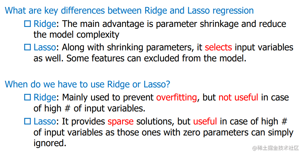
(1)Ridge Regression
For ridge regularised error is still a quadratic function of weights
1 2 ∑ n = 1 N ( t n − y ( x n , w ) ) 2 + λ 2 ∥ w ∥ 2 \frac{1}{2} \sum_{n=1}^{N}\left(t_{n}-y\left(\boldsymbol{x}_{n}, \boldsymbol{w}\right)\right)^{2}+\frac{\lambda}{2}\|\boldsymbol{w}\|^{2} 21∑n=1N(tn−y(xn,w))2+2λ∥w∥2
Finding gradient and setting to 0 again identifies system of linear equations with solution:(找到梯度,再设为0,就可以确定线性方程组的解)
w = ( λ I + Φ T Φ ) − 1 Φ T t \boldsymbol{w}=\left(\lambda \boldsymbol{I}+\boldsymbol{\Phi}^{T} \boldsymbol{\Phi}\right)^{-1} \boldsymbol{\Phi}^{T} \boldsymbol{t} w=(λI+ΦTΦ)−1ΦTt
Hence, can be solved directly or iteratively with (S)GD
Sidenote: Can derive ridge regression as Bayesian method by defining normal distribution prior distribution on parameters
(2)Lasso Regression
Problem: Lasso regularised error is not differentiable(不可微的). However, is still convex(凸).

Popular options:
-
Use gradient descent anyway with “sub-gradient”
-
Coordinate-wise descent
Key Differences: Ridge & Lasso
Bias & Variance decomposition 偏差-方差分解
- Variance and Standard Deviation 方差和标准差

- When the model has a high variance, you can try to train the model on a larger dataset or with smaller sets of features, but if the model has a high bias, they will not fix the problem, you can try to obtain new features
-
bias is a learner’s tendency to consistently learn the same wrong thing
-
variance is the tendency to learn random things irrespective of the real signal
-
noise 噪声表达了当前任务上任何学习算法所能达到的期望泛化误差下界,即学习问题本身的难度

Our goal is to minimize the generalisation error, which we have decomposed into the sum of a (squared) bias and a variance. As we shall see, there is a trade-off between bias and variance, with very flexible models having low bias and high variance, and relatively rigid models having high bias and low variance.
Linear Classification
分类与回归
The main difference between classification and regression tasks is the type of output variable, which is discrete for classification but continues for regression.
基础
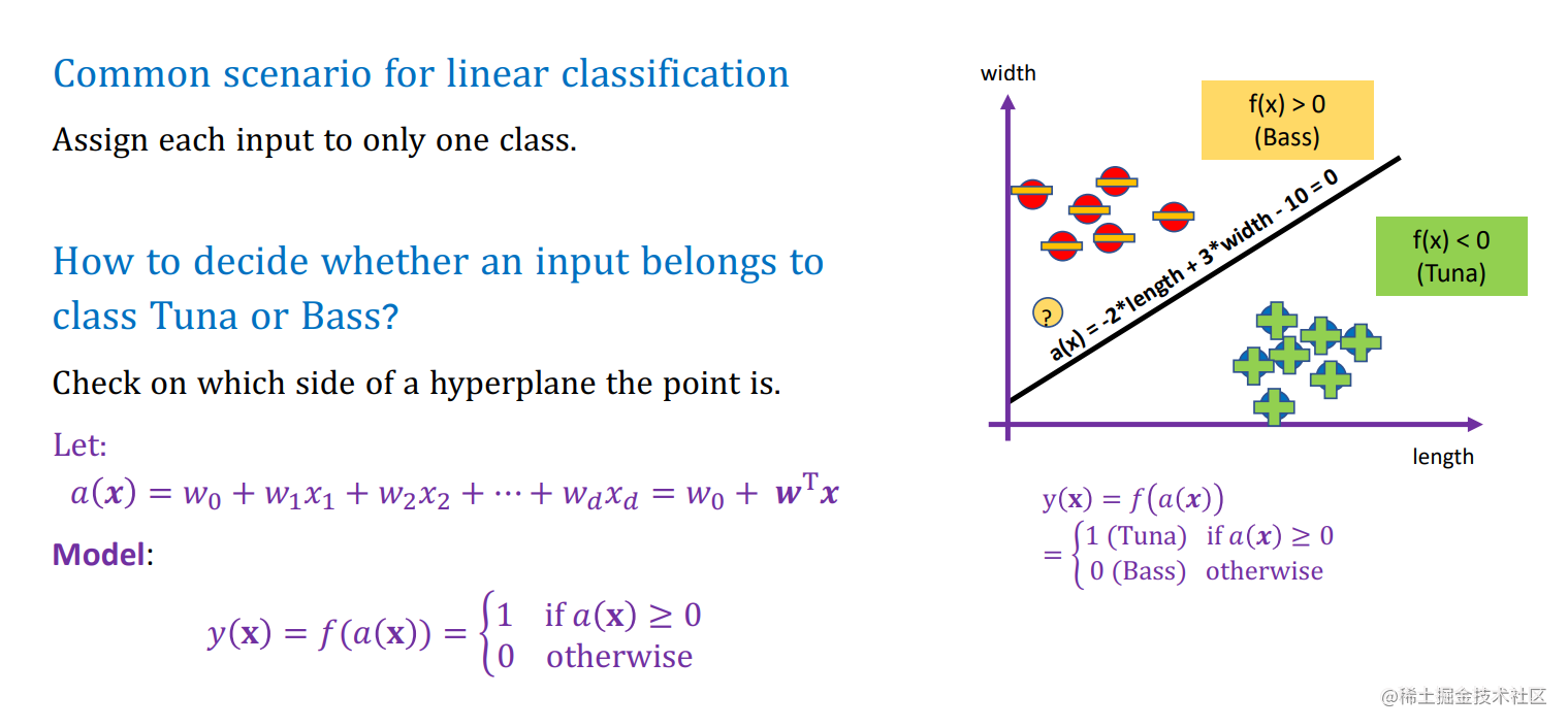
How to define a decision boundary?

How to decide whether an input belongs to class Tuna or Bass? Check on which side of a hyperplane the point is

分类方法
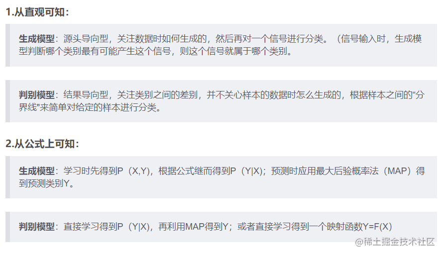
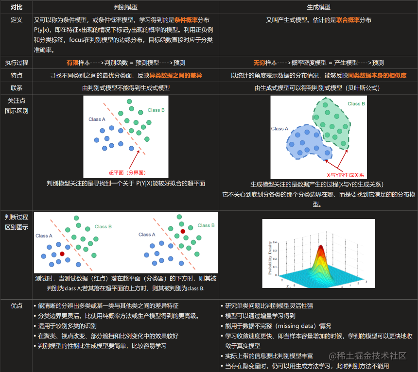
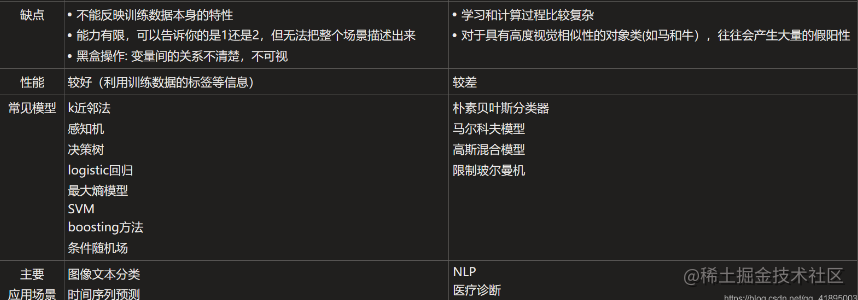
- 判别性模型 Discriminative Models:non-probabilistic models which directly assign the input X X X to a specific class C k C_{k} Ck . The simplest method to build a discriminant function is the Perceptron Algorithm. 直接将x输入到特别的类 C k C_{k} Ck
学习得到条件概率分布 P(y|x),即在特征 x 出现的情况下标记 y 出现的概率。(判 别模型就是直接学习条件概率分布 P(y∣x))。
这类模型的典型代表是 logistic 回归和 softmax 回归,它们直接对 p(y∣x)建模, 而不对 p(x,y)建模,即每一假设 x 服从何种概率分布。logistic 回归用于二分类问 题,它直接根据样本 x 估计出它是正样本的概率。
-
概率判别模型Probabilistic (Discriminative) Models 不是将输入分配到一个特定的类别,而是对一个给定的输入产生属于每个类别的概率 P ( c k ∣ x , w ) P(c_{k} \mid x,w) P(ck∣x,w)
-
概率生成模型 Probabilistic Generative Models learn the class-prior distribution and the class-conditional distribution and combine them based on the Bayes rule to get the class posterior, can be used to generate input variables

学习得到联合概率分布 P(x,y),即特征 x 和标记 y 共同出现的概率,然后求条件 概率分布。能够学习到数据生成的机制。(生成模型就是要学习 x 和 y 的联合概 率分布 P(x,y),然后根据贝叶斯公式来求得条件概率 P(y∣x),预测条件概率最大的y)。
常见的生成模型:朴素贝叶斯、隐马尔可夫模型
联合概率分布 joint probability distribution
条件概率分布 Conditional probability distribution
- Generative VS Discriminative
-
如果我们有生成式模型,我们可以生成合成数据 ,而如果我们只有鉴别式模型,就不能生成这样的数据
-
生成性模型通常有更多的参数。更多的参数会导致更多的复杂性,从而使模型容易出现各种问题,例如过拟合。
Generalized Linear Models 广义线性模型
线性回归模型:

为了能够获得分类问题所需的离散输出,我们通过对回归输出应用非线性函数 ,来概括线性回归模型:

Linear regression passes through an activation function and then obtains the classification result according to a threshold value, thus becoming linear classification;

Discriminative Models 判别性模型
两类判别函数 Two Class Discriminant Function

几何证明题

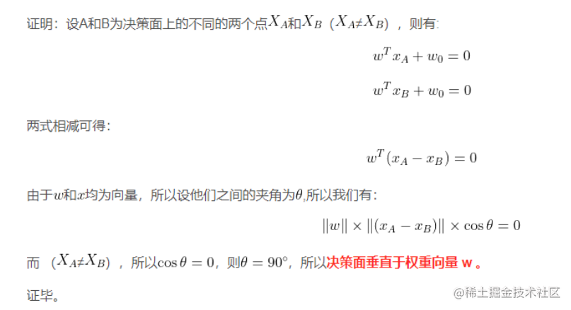
(1)证明决策面垂直于权重向量w 或 决策变量与w正交

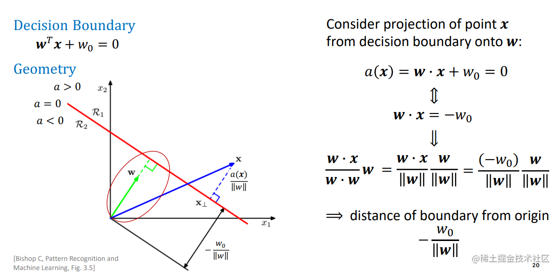
(2) 计算输入向量x在权重向量w上的投影大小
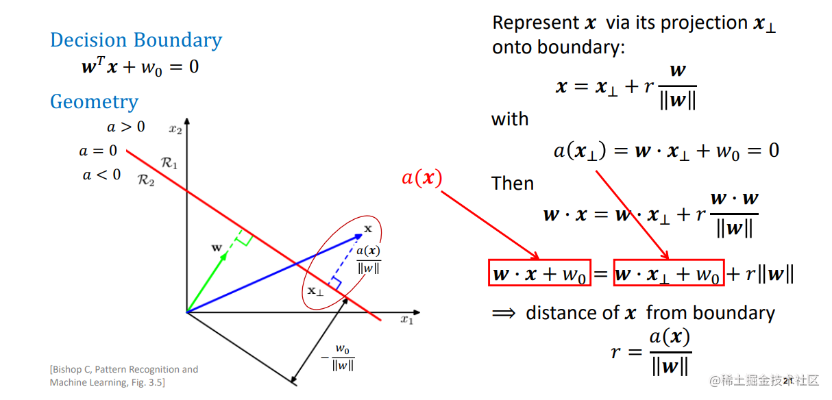
(3)输入向量x到决策面的距离向量为
Generalisation to Multiclass Problems
- One-versus-the-rest classifier 一对多法分类器
训练时依次把某个类别的样本归为一类,其他剩余的样本归为另一类,这样 k 个类别的样本就构造出了 k 个 SVM。分类时将未知样本分类为具有最大分类函数值的那类。 During training, the samples of a certain class are classified into one class, and the other remaining samples are classified into another class. Thus, K SVM are constructed from the samples of K classes. The unknown samples are classified into the class with the largest classification function value

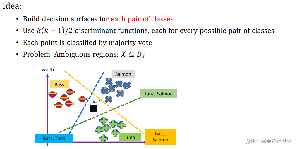
- One-versus-one classifier
其做法是在任意两类样本之间设计一个SVM,因此 k 个类别的样本就需要 设计 k(k-1)/2 个 SVM。当对一个未知样本进行分类时,最后得票最多的类别即为该未知样本的类别。Libsvm 中的多类分类就是根据这个方法实现的。 The method is to design an SVM between any two classes of samples, so K (k-1) / 2 SVM are required for K classes of samples. When an unknown sample is classified, the category with the most votes is the category of the unknown sample. The multi class classification in libsvm is implemented according to this method
3.Use K discriminant functions a k ( x ) a_{k}(x) ak(x)


The Perceptron Algorithm 感知机 硬分类且属于判别模型
- 感知机过程
The input of the perceptron is** the feature vector of the sample**, and the output is the** category of the sample**, taking + 1 and - 1 as two values.
The specific method is to introduce a multiplicative weight to each one-dimensional feature of the sample to express the importance of each feature, and then add a bias term to the sum of the products.
The results are sent to the symbolic function, and the samples are divided into two categories by using the binary characteristics of the symbolic function.
训练感知机的目标可以概括为:寻找合适的权值和偏置, 使得符号函数能够将样本尽量准确地分成两类。
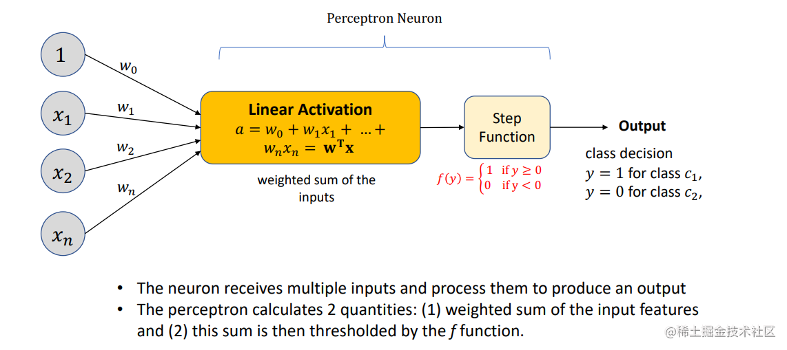
the nonlinear activation function f ( ) f( ) f() ⋅ is given by a step function
- 误差函数和误分类

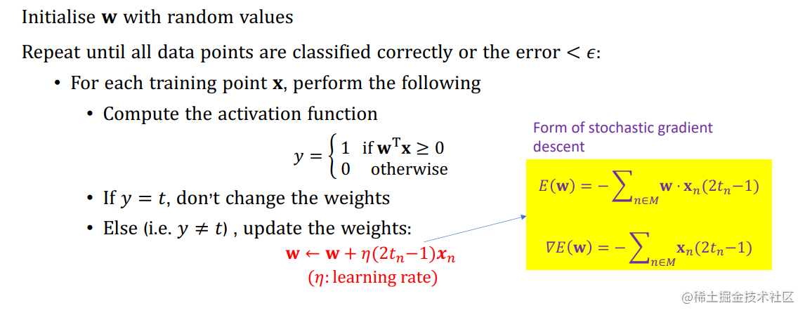
- 感知机的算法步骤

-
随着参数的变化,被正确修改的数据点可能会变成被错误分类的数据。As the parameters change, the data points that were correctly modified might change to being misclassified
-
用梯度下降法SGD更新参数
- Example

这里t是当前的分类


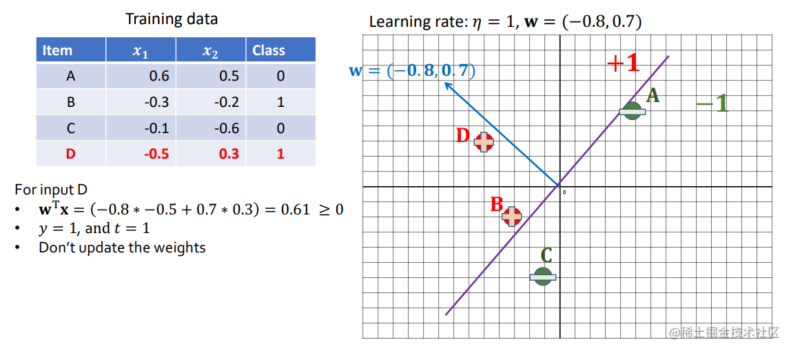

- 如果数据是线性可分离 linearly separable的,Perceptron保证能找到一个训练误差为0的参数向量。然而,该算法可能需要在数据集上进行太多的迭代才能收敛到一个完美的参数向量。
- 如果数据不是线性可分离的,Perceptron可能无法收敛。在这种情况下,它可能在一些权重向量中循环而不停止。
- Perceptron对初始化很敏感。如果他们以不同的顺序访问训练实例,两次运行可能产生不同的权重。
Probabilistic Discriminative Models 概率判别模型
概率判别模型使用广义线性模型来直接获得类的后验概率,并旨在通过最大似然来学习参数
- 逻辑回归Logistic Regression: 用于分类
- 梯度下降SGD: 学习模型参数
Logistic Regression
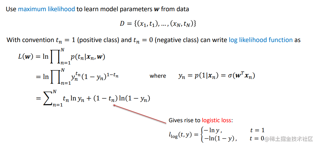
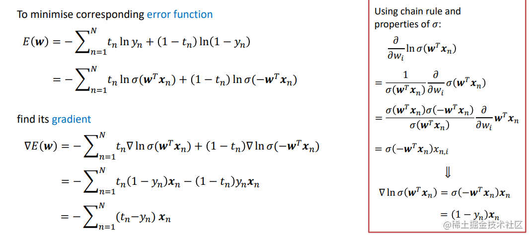
- Logistic回归使用线性函数来模拟两个类别(或一个与另一个)的对数几率。
- 参数化对数几率是广泛用于概率分类的方法(不仅仅是在线性模型)。
- 可解释的模型:输入权重的大小表示相应输入变量的重要性
- 警告:(随机)梯度下降法对于线性可分离的数据是不收敛的;原因是:会把权重的规范推到无穷大。
- 我们通常使用正则化来避免这种情况。
- 可以对多个类别进行泛化(使用被称为 "softmax "的sigmoid的变体)。
Gradient Descent
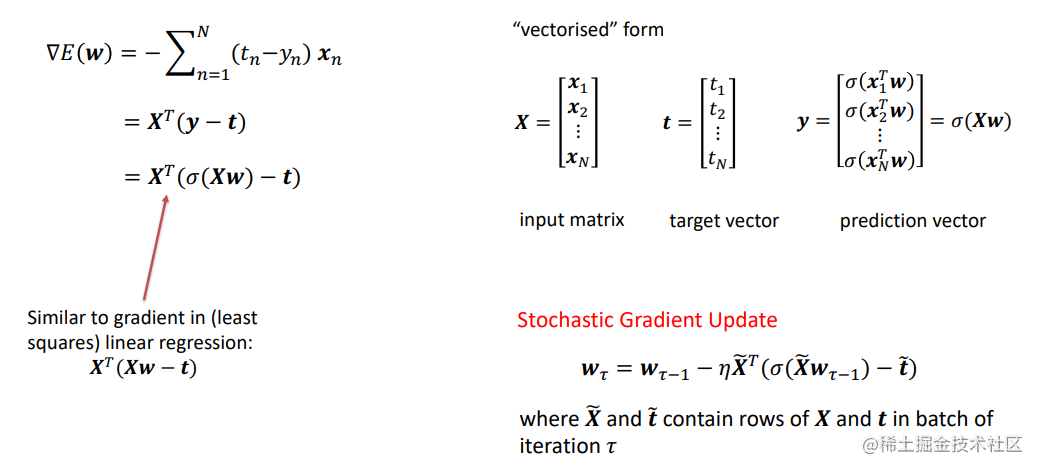
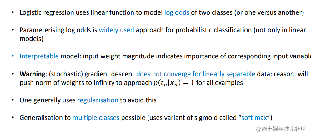
Logistic Regression 和 Linear Regression 区别与联系
-
一般 Linear Regression 是解决回归问题,而 Logistic Regression 是应用于分 类问题。 In general, Linear Regression is used to solve Regression problems, while Logistic Regression is applied to classification problems.
-
Logistic Regression 除了可以解决二分类问题外,还可以解决多分类问题 Logistic Regression can solve multiple classification problems in addition to binary classification problems.

Probabilistic Generative Models 概率生成模型
考试参考的题
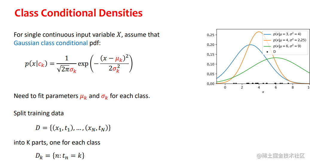
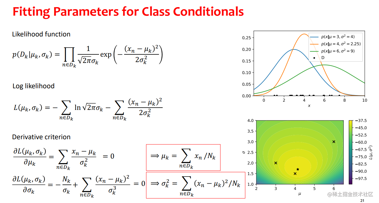

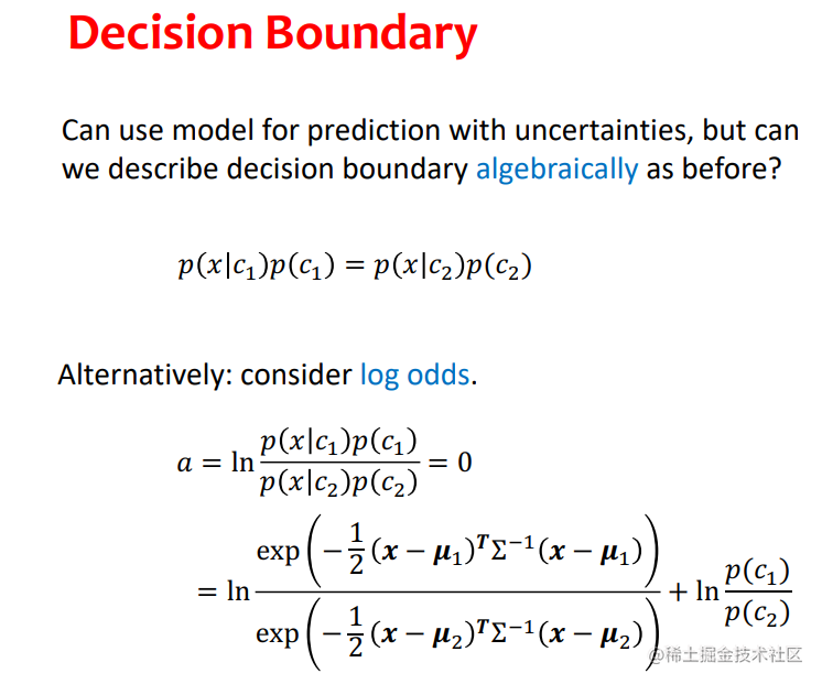
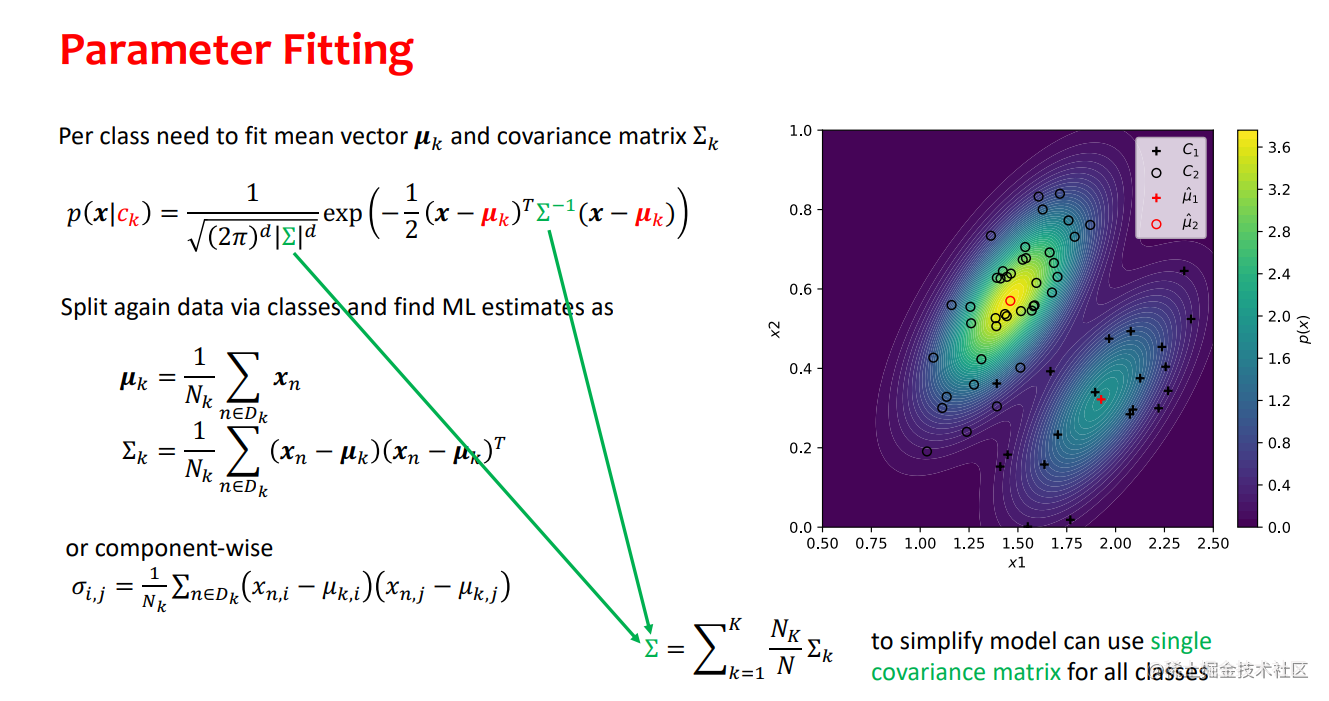

- 具有正态类条件密度的生成模型(贝叶斯分类器)是一个有吸引力的选择,因为它们允许以封闭形式找到ML参数,而无需昂贵的迭代算法。
- 然而,它们需要选择条件输入分布conditional input distributions(有时多变量正态可能不能很好地捕捉数据)
- 另外,如果不使用Naïve Bayes假设,有相对多的参数需要拟合
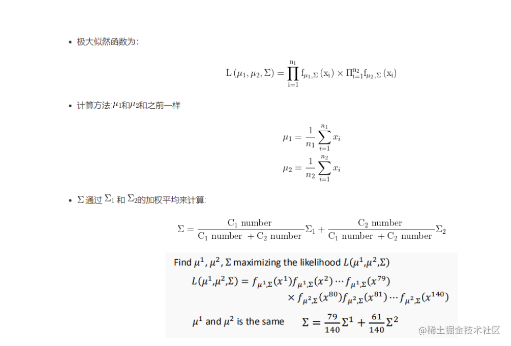
- 可以使用共享协方差shared covariance来减少参数的系数K
- 可以扩展到离散特征,通常与Naïve Bayes假设相结合,其中每个特征都被模拟为类条件下的伯努利或多项式随机变量。

分类过程中如何预防过拟合问题
➢ Cross fold validation
➢ Use more data for training
➢ Remove some characteristic values
➢ Stop training early
➢ Regularization
➢ Ensemble model fusion
Latent Variable Models
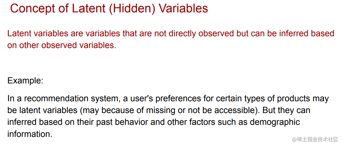
Clustering Methods
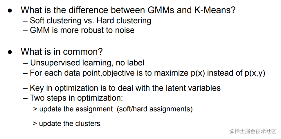
1: K-Means clustering (hard clustering)
2: Mixture models (soft clustering)
3: Spectral clustering (e.g., Normalized cuts, Graph Laplacian…)
4: Biclustering
Soft and hard clustering
Soft clustering: Data points may belong to one or more clusters, and the probability of belonging to each cluster is given.
Hard clustering: Data points belong to only one cluster
K-Means Algorithm
-
K-Means is sensitive to initial values – which means the different execution of K-means with different initial cluster centers may result in different solutions
-
K-Means is a non-probabilistic algorithm – which only supports hard-assignment – a data point can only be assigned to one and only one of the clusters


Recall MLE vs. MAP
-
Same points: a point estimate of the parameters
-
Different points: the assumption of the prior of parameters
-
When dealing with small scale data, MAP is superior than MLE if a good prior is chosen.
-
When dealing with big data, MAP $ \approx$ MLE, given the law of large numbers. Prior has a little effect in this case.
K-means的基本步骤

EM Algorithm
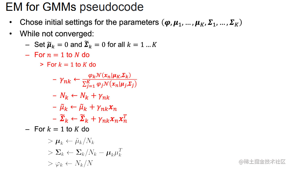
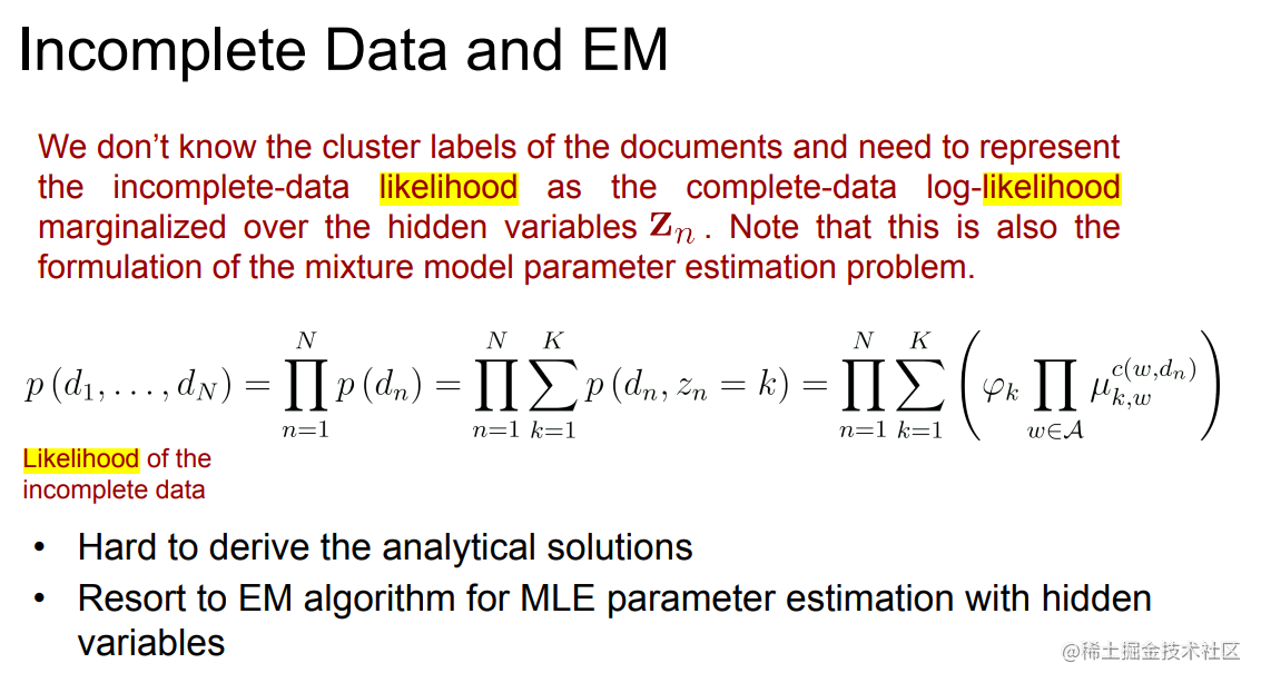
The goal of EM is to maximize the log likelihood of the observed data.
It maximizes the incomplete-data log-likelihood

基本步骤
1.Initialize the model parameters
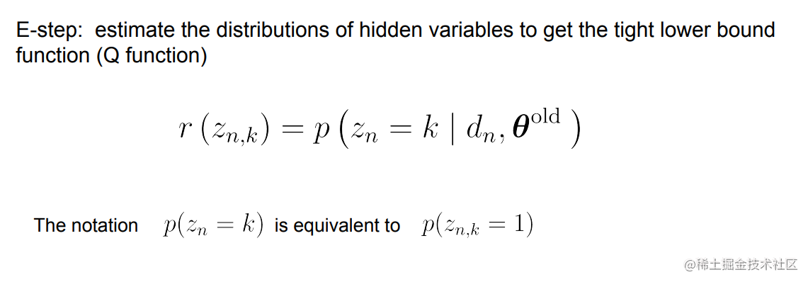
- E step
We use the current parameter values θ o l d \theta^{old} θold to find the posterior distribution of the latent variables given by p ( Z ∣ X , θ o l d ) p(Z \mid X, \theta_{old}) p(Z∣X,θold) . We then use this posterior distribution to find the expectation of the complete-data log likelihood evaluated for some general parameter value θ \theta θ .

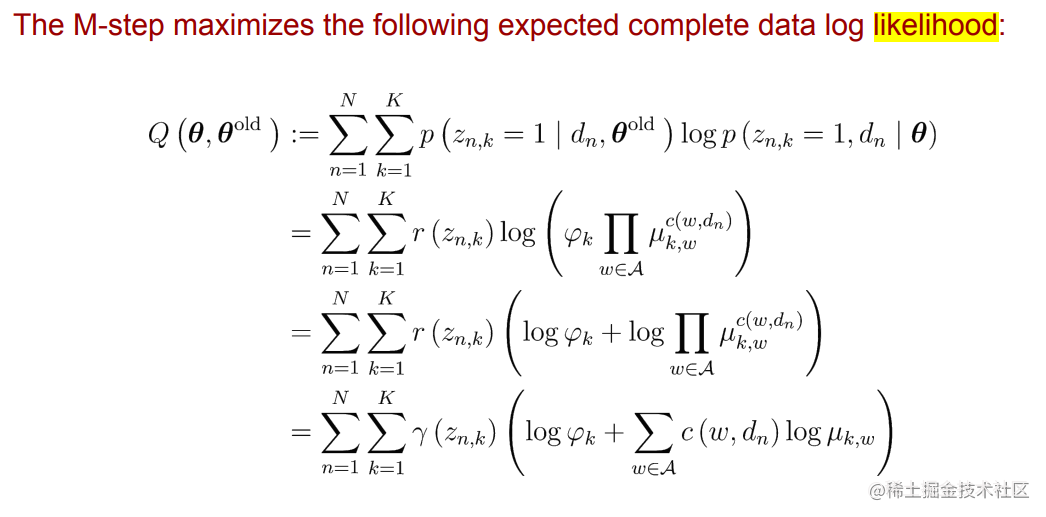
- M step
In the M step, we determine the revised parameter estimate θ n e w \theta^{new } θnew by maximising this function


GMM(EM 算法应用)
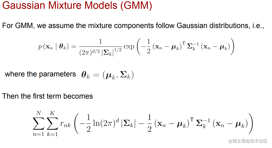
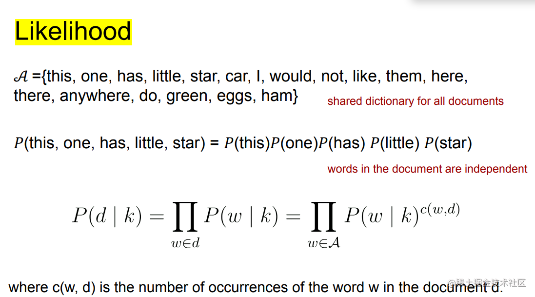
Document clustering 文本聚类(EM 算法应用)



Neural Networks 神经网络
**感知机和神经网络的区别 **
➢ 感知机使用的学习策略是梯度下降法 The learning strategy used by perceptron is gradient descent method
➢ 神经网络,在感知机基础上增加激活函数,loss 有交叉熵等 Neural network, adding activation function on the basis of perceptron, loss has cross entropy
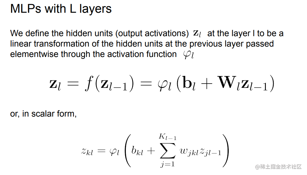
Multi-layer Perceptrons (MLPs)


Backpropagation VS Forwardpropagation 正向/反向传播
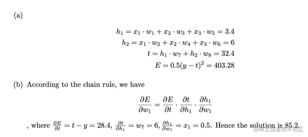
使用链式法则Chain Rule进行计算

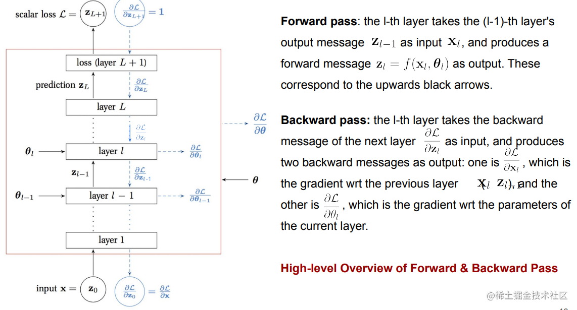

Feedforward process


Backpropagation process

Practice 参考中的题

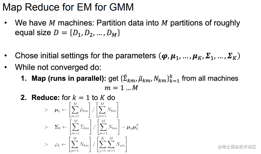
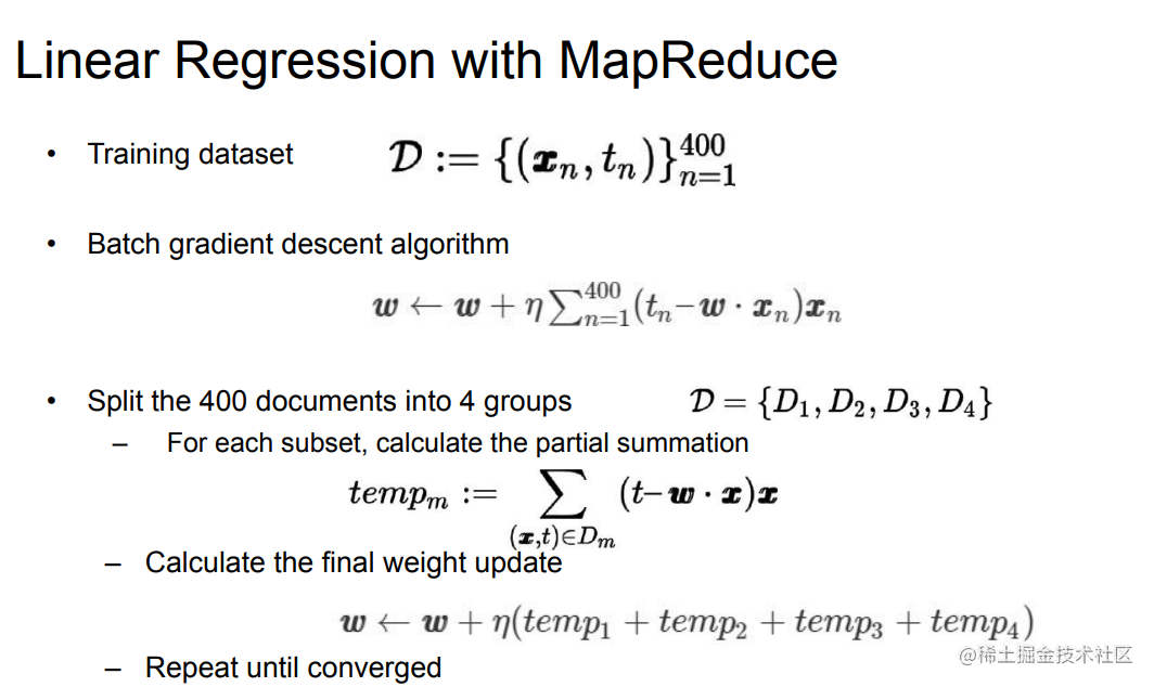
Scalable Machine Learning
MapReduce for Supervised Learning

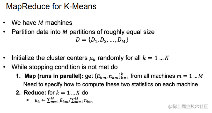
MapReduce for Supervised Learning
We need to calculate the distance of each data point x n x_{n} xn and the new center
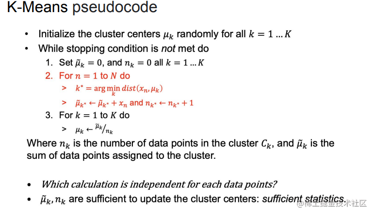
MapReduce for EM
