Simplex Method (单纯形方法)

学习目标：在本节中，我们将学习使用\(\textbf{单纯形法}\)解决线性规划最大化问题：(In this section, we will learn to solve linear programming maximization problems using the Simplex Method:)

1. 识别并建立标准的最大化形式的线性规划 (Identify and set up a linear program in standard maximization form)
2. 使用松弛变量将不等式约束转换为方程 (Convert inequality constraints to equations using slack variables)
3. 使用目标函数和松弛方程建立初始单纯形表 (Set up the initial simplex tableau using the objective function and slack equations)
4. 通过执行旋转操作找到最佳单纯形表 (Find the optimal simplex tableau by performing pivoting operations)
5. 从最佳单纯形表中识别最佳解决方案。(Identify the optimal solution from the optimal simplex tableau.)

在现实生活中，线性规划问题实际上包含数千个变量，并且由计算机解决(无法通过几何方法来解决，其针对两个变量的问题)。我们可以用代数方法解决这些问题，但效率不高。(In real life situations, linear programming problems consist of literally thousands of variables and are solved by computers. We can solve these problems algebraically, but that will not be very efficient.) 假设我们遇到一个有5个变量和10个约束的问题。通过选择五个方程和五个未知数的所有组合，我们可以找到所有角点，测试它们的可行性，并得出解(如果存在)。(Suppose we were given a problem with, say, 5 variables and 10 constraints. By choosing all combinations of five equations with five unknowns, we could find all the corner points, test them for feasibility, and come up with the solution, if it exists.) 但问题是，即使对于变量如此至少的问题，我们也会得到250多个角点，而测试每个点将非常繁琐。因此，我们需要一种具有系统性的算法并且可以为计算机编程的方法。该方法必须足够高效，这样，我们就不必再每个角点处评估目标函数。我们正好有一种方法，它被称为单纯形法。(But the trouble is that even for a problem with so few variables, we will get more than 250 corner points, and testing each point will be very tedious. So we need a method that has a systematic algorithm and can be programmed for a computer. The method has to be efficient enough so we wouldn't have to evaluate the objective function at each corner point. We have just such a method, and it is called the \(\textbf{Simplex Method}\).)

单纯形法是由乔治\(\cdot\)丹齐格博士在第二次世界大战期间发明的。他的线性规划模型帮助盟军解决了运输和调度问题。(The simplex method was developed during the Second World War by Dr.George Dantizg. His linear programming models helped the Allied forces with transportation and scheduling problems.)

单纯形法使用了一种非常有效的方法。它不计算每个点的目标函数值；相反，它从可行区域的一个角点开始，然后系统地从一个角点移动到另一个角点，同时在每个阶段改进目标函数的值。这个过程一直持续到找到最优解。(The simplex method uses an approach that is very efficient. It does not compute the value of the objective function at every point;instead, it begins with a corner point of the feasibility region where all the main variables are zero and then systematically moves from cornrt point to corner point, while improving the value of the objective function at each stage. The process continues until the optimal solution is found.)

为了学习单纯形法，我们尝试了一种相当不寻常的方法。我们首先列出算法，然后解决问题。我们在此过程中证明每个步骤背后的原因。彻底地证明超出了本节的范围。(To learn the simplex method, we try a rather unconventional approach. We first list the algorithm, and then work a problem. We justify the reasoning behind each step during the process. A thorough justification is beyond the scope of this section.)

首先，我们列出单纯形法的算法。(We first list the algorithm for the simplex method.)

1. 设定问题。即，写出目标函数和不等式约束。 (Set up the problem. That is, write the objective function and the inequality constraints.)
2. 将不等式转换为方程。这是通过为每个不等式添加一个松弛变量来完成的。(Convert the inequalities into equations. This ia done by adding one slack variable for each inequality.)
3. 构建初始单纯形表。将目标将函数写为底行。(Construct the initial simplex tableau. Write the objective function as the bottom row.)
4. 底行中最负的项来识别枢轴列。(The most negative entry in the bottom row identifies the pivot column.)
5. 计算商。通过将最右边的列除以在步骤4中识别的列来计算商。为零、负数或分母为零的商将被忽略。识别最小商所在的行。在步骤4中识别的列与在此步骤中识别的行的交点中的元素被定义为枢轴元素。(Calculate the quotients. The quotients are computed by dividing the far right column by the identified column in step 4. A quotient that is a zero, or a negative number, or that has a zero in the denominator, is ignored. The smallest quotient identifies a row. The element in the intersection of the column identified in Step 4 and the row identified in this step is identified as the pivot element.)
6. 执行枢轴化(消去法)以使此列中的所有其他项为零。这与我们使用高斯-乔丹方法的方式相同。(Perform pivoting to make all other entries in this column zero. This ia done the same way as we did with the Gauss-Jordan method.)
7. 当底行中没有负项时，我们就完成了；否则，我们从步骤4重新开始。(When there are no more negative entries in the bottom row, we are finished;otherwise,we start again from Step 4.)
8. 解释结果。(Read off the results. Get the variables using the columns with 1 and 0s.)

现在，我们用单纯形法来求解下面的例子。(Now, we use the simplex method to solve the following example.)

Niki有两份兼职工作，工作 A 和工作 B。她每周的工作时间总计不超过 \(12\) 小时。她已确定，在工作 A 上工作一个小时，她都需要 \(2\) 小时的准备时间，在工作 B 上工作的每个小时，她都需要 \(1\) 小时的准备时间，并且她不能花超过 \(16\) 小时的准备时间。如果她在工作 A 上每小时赚 \(40\) 美元，在工作 B 上每小时赚 \(30\) 美元，那么她每周应该在每份工作上工作多少小时才能使收入最大化？(这个问题当然很简单，用几何的方法就可以解决，但我们这里用这个例子来展示单纯形的工作原理。) (Niki holds two part-time jobs, Job A and Job B. She never wants to work more than a total of 12 hours a week. She has determined that for every hour she works at Job A, she needs 2 hours of preparation time, and for every hour she works at Job B, she needs one hour of preparation time, and she cannot spend more than 16 hours for preparation. If she makes 40 dollar an hour at Job A, and 30 dollar an hour at Job B, how many hours should she work per week at each job to maximize her income?)

答(Solution)：
在解决这个问题时，我们将遵循上面列出的算法。(In solving this problem, we will follow the algorithm listed above.)

步骤1 设定问题。写出目标函数和约束。由于单纯形法用于包含许多变量的问题，因此使用变量 \(x,y,z\) 等并不实际。我们使用符号 \(x_1\), \(x_2\), \(x_3\) 等。(Since the simplex method is used for problems that consist of many variables, it is not practical to use the variables \(x,y,z\) etc. We use symbols \(x_1\), \(x_2\), \(x_3\), and so on.)

设

• \(x_{1}\)=Niki 每周在 Job A 上工作的时间
• \(x_{2}\)=Niki 每周在 Job B 上工作的时间.
  习惯上选择要最大化的变量作为 \(Z\)。(It is customary to choose the variable that is to be maximized as \(Z\).)

\begin{split}
\max \quad &Z=40x_{1}+30x_{2}\\
s.t. \quad & x_{1}+x_{2}\le 12\\
\quad & 2x_{1}+x_{2}\le 16\\
\quad & x_{1}\ge 0; x_{2}\ge 0
\end{split}

步骤2 将不等式转换为方程。(Convert the inequalities into equations.)
例如，为了将不等式 转换为方程，我们添加一个非负的松弛变量 \(y_1\),(For example to convert the inequality \(x_1+x_2\le 12\)
into an equation, we add a non-negative variable \(y_{1}\),) 我们得到 (we get)

\[x_1+x_2+y_1=12, \]

其中，变量 \(y_1\) 弥补了不足，它表示 \(x_1+x_2\) 距离 \(12\) 的差值。(Here the variable \(y_{1}\) picks up the slack, and it represnts the amount by which \(x_1+x_2\) falls short of \(12\).) 在这个问题中，如果Niki的工作时间少于 \(12\) 小时，比如 \(10\)，那么 \(y_{1}\) 就是 \(2\)。稍后，当我们从单纯形表中读出最终解决方案时，松弛变量的值将标识未使用的量。(In this problem, if Niki works fewer than \(12\) hours, say 10, then \(y_{1}\) is \(2\). Later when we read off the final solution from the simplex table, the values of the slack variables will identify the unused amounts.)

我们重新写目标函数 \(Z=40x_{1}+30x_{2}\) 为 \(-40x_{1}-30x_{2}+Z=0\)。
添加松弛变量后，我们的问题读作（After adding the slack variables, our problem reads）
\begin{split}
\text{Objective function}\quad &-40x_{1}-30x_{2}+Z=0\\
\text{Subject to constraints:} \quad & x_{1}+x_{2}+y_{1}= 12\\
\quad & 2x_{1}+x_{2}+y_{2}=16\\
\quad & x_{1}\ge 0; x_{2}\ge 0
\end{split}

步骤3 构建初始的单纯形表格。(Construct the initial simplex tableau.) 每个不等式约束出现在其自己的行中。(非负约束不会作为单纯形表中的行出现)。将目标函数放在表格的最底行。(Each inequality constraint appears in its own row. The non-negativity constraints do not appear as rows in the simplex tableau. Write the objective function as the bottom row.)

现在不等式已转化为方程，我们可以将问题表示为一个称为初始单纯形表的增广矩阵，如下所示。(Now that the inequalities are converted into equations, we can represent the problem into an augmented matrix called the initial simplex tableau as follows.)

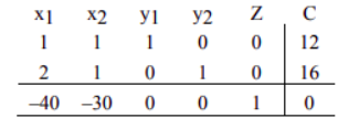
这里，竖线分割了方程的左右两侧。横线分割了约束和目标函数。并且方程的右边用列C表示。(Here the vertical line separates the left hand side of the equations from the right side. The horizontal line separates the constraints from the objective function. The right side of the equation is represented by the column C.)

读者需要观察到，该矩阵的最后四列看起来像方程组解的最终矩阵。(The reader needs to observe that the last four columns of this matrix look like the final matrix for the solution of a system of equations.) 如果我们任意选择\(x_1=0, x_2=0\), 我们得到(If we arbitrarily choose \(x_1=0\) and \(x_2=0\), we get)

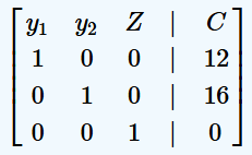
也就是：$$y_{1}=12, y_{2}=16, Z=0$$

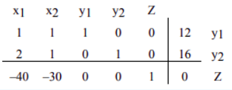
通过任意赋值某些变量，然后求解剩余变量而得到的解称为与表相关的基本解。因此，上述解是与初始单纯形表相关的基本解。我们可以在最后一列的右侧标记基本解变量，如下表所示。(The solution obtained by arbitrarily assigning values to some variables and then solving for the remaining variables is called the basic solution associated with the tableau. So the above solution is the basic solution associated with the initial simplex tableau. We can label the basic solution variable in the right of the last column as shown in the table below.)

步骤4 用底行中最负的项来识别枢轴列。

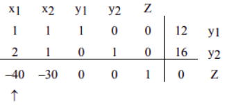
问题：为什么我们要选择最底行最负的项？(Why do we choose the most negative entry in the bottom row？)
答：底行中最负的项代表目标函数中的最大系数——该系数的输入将最快增加目标函数的值。(The most negative entry in the bottom row represents the largest coefficient in the objective function - the coefficient whose entry will increase the value of the objective function the quickest.) 单纯形法从一个角点开始，在这个角点上，所有主要变量（带有符号的变量，例如 \(x_1,x_2,x_3\) 等）都为零。然后，它从一个角点移动到相邻的角点，始终增加目标函数的值。在目标函数 \(Z=40x_1+30x_2\) 的情况下，增加 \(x_1\) 的值比增加 \(x_{2}\) 的值更有意义。变量 \(x_1\) 表示 Niki 在工作 A 上每周工作的小时数。由于工作 A 每小时支付 \(40\) 美元，而工作 \(B\) 每小时仅支付 \(30\) 美元，因此变量 \(x_1\) 每增加一个单位，目标函数就会增加 \(40\) 美元。(The simplex method begins at a corner point where all the main variables, the variables that have symbols such as \(x_1,x_2,x_3\) etc., are zero. It then moves from a corner point to the adjacent corner point always increasing the value of the objective function. In the case of the objective function \(Z=40x_1+30x_2\), it will make more sense to increase the value of \(x_1\) rather than \(x_2\). The variable \(x_1\) represents the number of hours per week Niki works at Job A. Since Job A pays \(40\) dollar per hour as opposed to Job II which pays only \(30\) dollar, the variable \(x_1\) will increase the objective function by 40 dollar for a unit of increase in the variable \(x_1\).)

步骤5

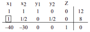
两个商 \(12\) 和 \(8\) 中最小的那个是 \(8\)。因此确定了第 \(2\) 行。第 \(1\) 列和第 \(2\) 行的交点是项目 \(2\)，该条目已突出显示。这是我们的枢轴元素。(The smallest of the two quotients, \(12\) and \(8\), is \(8\). Therefore row \(2\) is identified. The intersection of column \(1\) and row \(2\) is the entry \(2\), which has been highlighted. This is our pivot element.)
问：为什么我们要求商，为什么最小的商可以确定一行？(Question: Why do we find quotients, and why does the smallest quotient identify a row?)
答：当我们选择最底行中最负的项时，我们试图通过引入变量 \(x_1\)来增加目标函数的值。但我们不能为 \(x_1\) 选择任意值。我们可以让 \(x_1=100\) 吗？绝对不行！这是因为 Niki 从来不想在两份工作上工作超过 \(12\) 个小时：\(x_{1}+x_{2}\le 12\)。我们可以让 \(x_{1}=12\) 吗？同样，答案是否定的，因为工作 A 的准备时间是工作时间的两倍。由于 Niki 从来不想花超过 \(16\) 个小时进行准备，因此她可以工作的最长时间为 \(16÷2=8\)。

现在我们明白了计算商的目的；使用商来识别枢轴元素可确保我们不违反约束。(Now we see the purpose of computing the quotients; using the quotients to identify the pivot element guarantees that we do not violate the constraints.)

问：为什么要确定枢轴元素？(Question: Why do we identify the pivot element?)
答：正如我们前面提到的，单纯形法从一个角点开始，然后移动到下一个角点，始终改善目标函数的值。通过改变变量的单位数来改善目标函数的值。我们可以增加一个变量的单位数，同时丢弃另一个变量的单位。旋转使我们能够做到这一点。（As we have mentioned earlier, the simplex method begins with a corner point and then moves to the next corner point always improving the value of the objective function. The value of the objective function is improved by changing the number of units of the variables. We may add the number of units of one variable, while throwing away the units of another. Pivoting allows us to do just that.）

被添加单位的变量称为进入变量，被替换单位的变量称为离开变量。上表中的进入变量是 \(x_{1}\)，由最底行中最负的项标识。离开变量 \(y_{2}\) 由所有商中的最小商识别。通俗讲就是Niki应该更多地将时间投入到工作A中了，并且减少准备的时间。

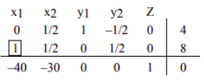
步骤6 执行旋转以使此列中的所有其他条目变为零。(Perform pivoting to make all other entries in this column zero.) 旋转是在枢轴元素的位置获得 \(1\)，然后将该列中的所有其他条目变为零的过程。所以现在我们的工作是通过将整个第二行除以 \(2\) 来使枢轴元素变为 \(1\)。结果如下。
(Pivoting is a process of obtaining a \(1\) in the location of the pivot element, and then making all other entries zeros in that column. So now our job is to make our pivot element a \(1\) by dividing the entire second row by \(2\). The result follows.)

为了在枢轴元素上方的第一个条目中获得零，我们将第二行乘以 \(-1\)，并将其添加到第 \(1\) 行。(To obtain a zero in the entry first above the pivot element, we multiply the second row by \(-1\) and add it to row \(1\). We get)

为了使枢轴下方的元素变为零，我们将第二行乘以 \(40\)，然后将其添加到最后一行。(To obtain a zero in the element below the pivot, we multiply the second row by 40 and add it to the last row.)

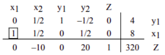
现在我们确定与该表相关的基本解决方案。如果我们写出增广矩阵，其左侧是一个列中有一个 \(1\) 而其他所有元素均为零的矩阵，我们得到以下矩阵，它陈述了同样的事情。(We now determine the basic solution associated with this tableau. By arbitrarily choosing \(x_2=0\) and \(y_2=0\), we obtain \(x_1=8, y_1=4, Z=320\). If we write the augmented matrix, whose left side is a matrix with columns that have one \(1\) and all other entries zeros, we get the following matrix stating the same thing.)

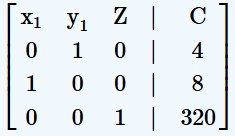
我们可以重新表述与该矩阵相关的解决方案。在游戏的这个阶段，如果 Niki 在工作 A 上工作 \(8\) 小时，而在工作 B 上不工作，她的利润 Z 将为 \(320\) 美元。这里 \(y_1=4, y_2=0\) 意味着她将剩下 \(4\) 小时的工作时间，没有准备时间。(We can restate the solution associated with this matrix as \(x_=8, x_2=0, y_1=4, y_2=0, Z=320\). At this stage of the game, it reads that if Niki works \(8\) hours at Job A, and no hours at Job B, her profit Z will be \(320\) dollar. Here \(y_1=4, y_2=0\) mean that she will be left with \(4\) hours of working time and no preparation time.)

步骤7 当底行中不再有负数条目时，我们就完成了；否则，我们从步骤 \(4\) 重新开始。(When there are no more negative entries in the bottom row, we are finished; otherwise, we start again from step \(4\).)

底行中不再有负数条目，因此我们已经完成。(We no longer have negative entries in the bottom row, therefore we are finished.)

问：为什么底行没有负数项就意味着完成了任务？(Why are we finished when there are no negative entries in the bottom row?)
答：答案就在最下面一行。最下面一行对应的是以下等式：(The answer lies in the bottom row. The bottom row corresponds to the equation:)

\[0x_1+0x_2+20y_1+10y_2+Z=400 \quad \text{or} \]

\[Z=400-20y_1-10y_2 \]

由于所有变量都是非负的，\(Z\) 所能达到的最高值是 \(400\)，而且只有当 \(y_1\) 和 \(y_2\)
为零时才会发生这种情况。(Since all variables are non-negative, the highest value \(Z\) can ever achieve is \(400\), and that will happen only when \(y_1\) and \(y_2\) are zero.)

步骤8. 解释结果(Read off your answers.)
现在我们读出答案，即确定与最终单纯形表相关的基本解决方案。再次，我们查看具有 \(1\) 且所有其他条目为零的列。由于标记为 \(y_1\) 和 \(y_2\) 的列不是这样的列，我们任意选择 \(y_1=0\) 和 \(y_2=0\)，我们得到(We now read off our answers, that is, we determine the basic solution associated with the final simplex tableau. Again, we look at the columns that have a 1 and all other entries zeros. Since the columns labeled \(y_1\)
and \(y_2\) are not such columns, we arbitrarily choose \(y_1=0\), and \(y_2=0\), and we get)

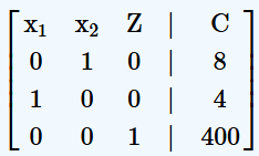
矩阵读取为 \(x_1=4,x_2=8,Z=400\)。

最终解决方案是，如果 Niki 在工作 A 上工作 \(4\) 小时，在工作 B 上工作 \(8\) 小时，她的收入将最大化为 \(400\) 美元。由于两个松弛变量均为零，这意味着她将用尽所有工作时间以及准备时间，不会剩下任何时间。(The final solution says that if Niki works 4 hours at Job A and 8 hours at Job B, she will maximize her income to 400 dollar. Since both slack variables are zero, it means that she would have used up all the working time, as well as the preparation time, and none will be left.)

至此我们已经分析了单纯形法的基本工作原理。

如果遇到(一般都是)最小化的问题，我们首先要通过下面的过程转换为一个最大化问题，然后就可以采用上面的单纯形法进行操作了。

再次提醒读者，在标准最小化问题中，所有约束都采用 \(ax+by\ge c\) 的形式。(Once again, we remind the reader that in the standard minimization problems all constraints are of the form \(ax+by\ge c\).)

解决这些问题(最小化问题)的程序是由约翰·冯·诺依曼博士开发的。它涉及解决一个称为对偶问题的相关问题。每个最小化问题都对应一个对偶问题。对偶问题的解用于找到原始问题的解。对偶问题是一个最大化问题，我们在上一节中学习了如何解决它。我们首先用单纯形法解决对偶问题。(The procedure to solve these problems was developed by Dr. John Von Neuman. It involves solving an associated problem called the dual problem. To every minimization problem there corresponds a dual problem. The solution of the dual problem is used to find the solution of the original problem. The dual problem is a maximization problem, which we learned to solve in the last section. We first solve the dual problem by the simplex method.)

然后，从最终的单纯形表中，我们提取原始最小化问题的解。(From the final simplex tableau, we then extract the solution to the original minimization problem.
)

然而，在进一步讨论之前，我们首先学习将最小化问题转换为其对应的最大化问题，称为其对偶问题。（Before we go any further, however, we first learn to convert a minimization problem into its corresponding maximization problem called its dual.）

例二(Example 2) 将以下最小化问题转换为其对偶问题。(Convert the following minimization problem into its dual.)

\begin{split}
\text{Minimize}\quad &Z=12x_1+16x_2\\
\text{Subject to:} \quad & x_{1}+2x_{2}\ge 40\\
\quad & x_{1}+x_{2}\ge 30\\
\quad & x_{1}\ge 0; x_{2}\ge 0
\end{split}

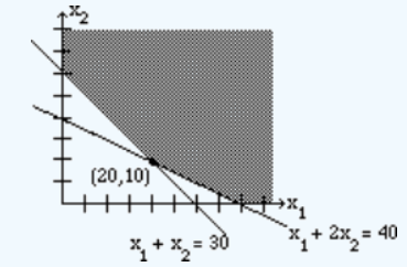
解(Solution): 为了实现我们的目标，我们首先将该问题表示为以下矩阵。(To achieve our goal, we first express our problem as the following matrix.)

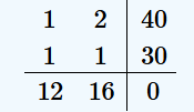
观察一下，这个表看起来像是一个没有松弛变量的初始单纯形表。接下来，我们写一个矩阵，其列是这个矩阵的行，行是该矩阵的列。这样的矩阵称为原始矩阵的转置。我们得到：（Observe that this table looks like an initial simplex tableau without the slack variables. Next, we write a matrix whose columns are the rows of this matrix, and the rows are the columns. Such a matrix is called a transpose of the original matrix. We get:）

与上述矩阵相关的下列最大化问题称为其对偶问题。(The following maximization problem associated with the above matrix is called its dual.)
\begin{split}
\text{Maximize}\quad &Z=40y_1+30y_2\\
\text{Subject to:} \quad & y_{1}+y_{2}\le 12\\
\quad & 2y_{1}+y_{2}\le 16\\
\quad & y_{1}\ge 0; y_{2}\ge 0
\end{split}

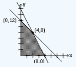
请注意，我们选择变量为 \(y\) 而不是 \(x\)，以区分这两个问题。（Note that we have chosen the variables as \(y\)'s, instead of \(x\)'s, to distinguish the two problems.）

最优解位于最终矩阵最底行与松弛变量对应的列中，目标函数的最小值与对偶的最大值相同。(The optimal solution is found in the bottom row of the final matrix in the columns corresponding to the slack variables, and the minimum value of the objective function is the same as the maximum value of the dual.)

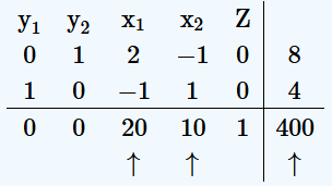
我们重新表述解决方案如下：(We restate the solution as follows:)
最小化问题在角点 (20, 10) 处具有最小值 400。 (The minimization problem has a minimum value of 400 at the corner point (20, 10)).

用单纯形法求解最小化问题 (Minimization by the Simplex Method)

• 设定问题 (Set up the problem.)
• 矩阵的行代表约束，最底行代表目标函数 (Write a matrix whose rows represent each constraint with the objective function as its bottom row.)
• 将得到的矩阵转置 (Write the transpose of this matrix by interchanging the rows and columns.)
• 写出转置对应的对偶问题 (Now write the dual problem associated with the transpose.)
• 用单纯形法求解得到的对偶问题 (Solve the dual problem by the simplex method.)
• 最优解位于最终矩阵最底行与松弛变量对应的列中，目标函数的最小值与对偶的最大值相同。(The optimal solution is found in the bottom row of the final matrix in the columns corresponding to the slack variables, and the minimum value of the objective function is the same as the maximum value of the dual.)

至此，通过变换，最小化问题也可由单纯形法去求解

然而，正如网上有人提到的一些关于单纯形法的问题(这也是每一个有好奇心的人都会自然想到的问题)：我们总是被告知单纯形算法是用于解决线性规划问题。(We are always told that the Simplex Algorithm is meant for solving linear equations with linear constraints.)

但是，如果我们将单纯形算法应用于更适合内点法等算法的典型非线性问题，其性能会有多差？(But how badly would the Simplex Algorithm perform if we implemented it on a typical non-linear problem that is better suited for algorithms such as the Interior Point Method?)

例如，单纯形算法“扫描”由所有方程和约束相交形成的外部表面上的不同顶点 - 我不确定由非线性方程和非线性约束形成的表面是否会有顶点？(For instance, the Simplex Algorithm "scans" different vertices on the exterior surface made by the intersection of all equations and constraints - I am not sure if the surface made by non-linear equations and non-linear constraints would even have vertexes?)

为了论证的目的，如果有人坚持在非线性问题上使用单纯形算法，这会立即失败吗？或者它理论上仍然可以返回可接受的答案，但这个答案不太可能是真正的最优答案？(For argument sake, if someone insisted on using the Simplex Algorithm on a non-linear problem, would this fail instantly? Or could it still in theory return an acceptable answer, but it would be unlikely that this answer was the true optimal?)

下面是一些有价值的回答 (Here are some valuable responses.)。

将单纯形法扩展到具有线性或线性化约束的非线性规划称为有效集方法。序列线性规划 (SLP) 和序列二次规划 (SQP) 是此类方法的典型示例，它们围绕约束的顶点移动，而不是像内点法 (IPM) 那样穿过内部。实施良好的 SQP 在数值上更稳健，并且在许多问题上可能比 IPM 更快。(Extension of the Simplex Method to Nonlinear Programs having linear or linearized constraints is called an Active Set method. Sequential Linear Programming (SLP) and Sequential Quadratic Programming (SQP) are notable examples of such methods, which move around vertices of the constraints, rather than cutting through the interior, as Interior-Point Methods (IPM) do. Well-implemented SQP can be more numerically robust and may be faster than IPM on many problems.)

应用于二次规划的有效集方法有时被称为单纯形法，即使它们与应用于线性规划的单纯形算法并不完全相同。(Active Set methods applied to Quadratic Programming are sometimes referred to as Simplex, even though they are not exactly the same as the Simplex Algorithm applied to Linear Programs.)

有两点(There are two points to this)：
单纯形算法的收敛依赖于始终可以在顶点中找到最佳解决方案的事实。这对于非线性问题并不成立（例如，考虑 \(\min x^2\), 其中 \(x\in [−1, 1]\))。如果算法无法收敛，那么在实践中它将如何工作？
单纯形的强大之处在于求解线性方程组。但如果问题是非线性的，那么您必须求解非线性方程组，这从计算、算法和数值的角度来看都是有问题的。所以在我看来，开箱即用的单纯形是行不通的。您可能会争辩说，您始终可以构建线性内部或外部 McCormick 松弛，这样单纯形就可以再次使用，但这无法与编写良好的内部点法相媲美。(The convergence of the Simplex algorithm relies on the fact that an optimal solution can always be found in a vertex. This does not hold for non-linear problems (consider e.g. \(\min x^2\), where \(x\in [−1, 1]\)). If an algorithm cannot converge, how would this then work in practice? The power of simplex method is based on solving sets of linear equations. But if the problem is non-linear, then you have to solve sets of non-linear equations which is problematic from a computational, algorithmic and numeric standpoint. So in my opinion using Simplex out of the box will not work. You could argue that you can always construct a linear inner or outer McCormick relaxation such that Simplex becomes usable again, but this will not compete with a well-written Interior Point method.)