前言

在Apollo星火计划学习笔记——Apollo路径规划算法原理与实践与【Apollo学习笔记】——Planning模块讲到……Stage::Process的PlanOnReferenceLine函数会依次调用task_list中的TASK，本文将会继续以LaneFollow为例依次介绍其中的TASK部分究竟做了哪些工作。由于个人能力所限，文章可能有纰漏的地方，还请批评斧正。

在modules/planning/conf/scenario/lane_follow_config.pb.txt配置文件中，我们可以看到LaneFollow所需要执行的所有task。

stage_config: {stage_type: LANE_FOLLOW_DEFAULT_STAGEenabled: truetask_type: LANE_CHANGE_DECIDERtask_type: PATH_REUSE_DECIDERtask_type: PATH_LANE_BORROW_DECIDERtask_type: PATH_BOUNDS_DECIDERtask_type: PIECEWISE_JERK_PATH_OPTIMIZERtask_type: PATH_ASSESSMENT_DECIDERtask_type: PATH_DECIDERtask_type: RULE_BASED_STOP_DECIDERtask_type: SPEED_BOUNDS_PRIORI_DECIDERtask_type: SPEED_HEURISTIC_OPTIMIZERtask_type: SPEED_DECIDERtask_type: SPEED_BOUNDS_FINAL_DECIDERtask_type: PIECEWISE_JERK_SPEED_OPTIMIZER# task_type: PIECEWISE_JERK_NONLINEAR_SPEED_OPTIMIZERtask_type: RSS_DECIDER

本文将继续介绍LaneFollow的第10个TASK——SPEED_BOUNDS_PRIORI_DECIDER

SPEED_BOUNDS_PRIORI_DECIDER功能简介

动态规划规划目标

• 加速度尽可能小
• 离障碍物纵向距离尽可能远
• 满足车辆加减速度要求
• 满足限速要求

产生粗糙速度规划曲线

SPEED_BOUNDS_PRIORI_DECIDER相关配置

modules/planning/conf/planning_config.pb.txt

default_task_config: {task_type: SPEED_HEURISTIC_OPTIMIZERspeed_heuristic_optimizer_config {default_speed_config {unit_t: 1.0dense_dimension_s: 101dense_unit_s: 0.1sparse_unit_s: 1.0speed_weight: 0.0accel_weight: 10.0jerk_weight: 10.0obstacle_weight: 1.0reference_weight: 0.0go_down_buffer: 5.0go_up_buffer: 5.0default_obstacle_cost: 1e4default_speed_cost: 1.0e3exceed_speed_penalty: 1.0e3low_speed_penalty: 10.0reference_speed_penalty: 10.0keep_clear_low_speed_penalty: 10.0accel_penalty: 1.0decel_penalty: 1.0positive_jerk_coeff: 1.0negative_jerk_coeff: 1.0max_acceleration: 2.0max_deceleration: -4.0spatial_potential_penalty: 1.0e2}lane_change_speed_config {unit_t: 1.0dense_dimension_s: 21dense_unit_s: 0.25sparse_unit_s: 1.0speed_weight: 0.0accel_weight: 10.0jerk_weight: 10.0obstacle_weight: 1.0reference_weight: 0.0go_down_buffer: 5.0go_up_buffer: 5.0default_obstacle_cost: 1e4default_speed_cost: 1.0e3exceed_speed_penalty: 1.0e3low_speed_penalty: 10.0reference_speed_penalty: 10.0keep_clear_low_speed_penalty: 10.0accel_penalty: 1.0decel_penalty: 1.0positive_jerk_coeff: 1.0negative_jerk_coeff: 1.0max_acceleration: 2.0max_deceleration: -2.5spatial_potential_penalty: 1.0e5is_lane_changing: true}}
}

modules/planning/proto/task_config.proto

// SpeedHeuristicOptimizerConfigmessage SpeedHeuristicOptimizerConfig {optional DpStSpeedOptimizerConfig default_speed_config = 1;optional DpStSpeedOptimizerConfig lane_change_speed_config = 2;
}message DpStSpeedOptimizerConfig {optional double unit_t = 1 [default = 1.0];optional int32 dense_dimension_s = 2 [default = 41];optional double dense_unit_s = 3 [default = 0.5];optional double sparse_unit_s = 4 [default = 1.0];optional double speed_weight = 10 [default = 0.0];optional double accel_weight = 11 [default = 10.0];optional double jerk_weight = 12 [default = 10.0];optional double obstacle_weight = 13 [default = 1.0];optional double reference_weight = 14 [default = 0.0];optional double go_down_buffer = 15 [default = 5.0];optional double go_up_buffer = 16 [default = 5.0];// obstacle cost configoptional double default_obstacle_cost = 20 [default = 1e10];// speed cost configoptional double default_speed_cost = 31 [default = 1.0];optional double exceed_speed_penalty = 32 [default = 10.0];optional double low_speed_penalty = 33 [default = 2.5];optional double reference_speed_penalty = 34 [default = 1.0];optional double keep_clear_low_speed_penalty = 35 [default = 10.0];// accel cost configoptional double accel_penalty = 40 [default = 2.0];optional double decel_penalty = 41 [default = 2.0];// jerk cost configoptional double positive_jerk_coeff = 50 [default = 1.0];optional double negative_jerk_coeff = 51 [default = 300.0];// other constraintoptional double max_acceleration = 60 [default = 4.5];optional double max_deceleration = 61 [default = -4.5];// bufferoptional double safe_time_buffer = 70 [default = 3.0];optional double safe_distance = 71 [default = 20.0];// spatial potential cost config for minimal time traversaloptional double spatial_potential_penalty = 80 [default = 1.0];optional bool is_lane_changing = 81 [default = false];
}

SPEED_BOUNDS_PRIORI_DECIDER流程

apollo Planning中用二次规划（PIECEWISE_JERK_SPEED_OPTIMIZER）或非线性规划（PIECEWISE_JERK_NONLINEAR_SPEED_OPTIMIZER）进行最后st曲线的优化，然而这种优化方法面对非凸问题就难以求出最优解了，所以在最后规划之前需要用一个粗的速度规划将非凸问题转化为凸问题。apollo中用了动态规划算法作为速度规划中非凸到凸问题的转化。

动态规划——通过把原问题分解为相对简单的子问题，再根据子问题的解来求解出原问题解的方法

状态转移方程
f ( P ) = min ⁡ { f ( R ) + w R → P } f(P) = \min \{ f(R) + {w_{R \to P}}\} f(P)=min{f(R)+wR→P​}
动态规划算法有两个核心概念：状态和状态转移方程。状态表示问题的一个局面或子问题的解，状态转移方程描述从一个状态到另一个状态的转移过程，其中每个状态都只与前面的几个状态相关。通过状态转移方程，我们可以得到所有可能的状态，从而得到问题的最优解。

基于动态规划的速度规划的流程如下：

1. 对路程和时间进行采样
2. 设计状态转移方程（cost计算）
3. 回溯找到最优S-T曲线

---

SPEED_HEURISTIC_OPTIMIZER的程序入口在modules/planning/tasks/optimizers/path_time_heuristic/path_time_heuristic_optimizer.cc中，首先来看Process部分：

Status PathTimeHeuristicOptimizer::Process(const PathData& path_data, const common::TrajectoryPoint& init_point,SpeedData* const speed_data) {init_point_ = init_point;// 检查if (path_data.discretized_path().empty()) {const std::string msg = "Empty path data";AERROR << msg;return Status(ErrorCode::PLANNING_ERROR, msg);}// 搜索ST图if (!SearchPathTimeGraph(speed_data)) {const std::string msg = absl::StrCat(Name(), ": Failed to search graph with dynamic programming.");AERROR << msg;RecordDebugInfo(*speed_data, reference_line_info_->mutable_st_graph_data()->mutable_st_graph_debug());return Status(ErrorCode::PLANNING_ERROR, msg);}RecordDebugInfo(*speed_data,reference_line_info_->mutable_st_graph_data()->mutable_st_graph_debug());return Status::OK();
}

可以看到，Process的输入为const PathData& path_data、const common::TrajectoryPoint& init_point、SpeedData* const speed_data。

同时，Process主要调用了SearchPathTimeGraph函数，接着来看该函数的实现：

首先根据是否换道选择配置文件，接着构建st_graph，类型为GriddedPathTimeGraph，最后调用Search()搜索出粗略的可行路线。

bool PathTimeHeuristicOptimizer::SearchPathTimeGraph(SpeedData* speed_data) const {// 根据是否换道选择配置文件const auto& dp_st_speed_optimizer_config =reference_line_info_->IsChangeLanePath()? speed_heuristic_optimizer_config_.lane_change_speed_config(): speed_heuristic_optimizer_config_.default_speed_config();// 初始化GriddedPathTimeGraph类对象 st_graphGriddedPathTimeGraph st_graph(reference_line_info_->st_graph_data(), dp_st_speed_optimizer_config,reference_line_info_->path_decision()->obstacles().Items(), init_point_);// 搜索ST图if (!st_graph.Search(speed_data).ok()) {AERROR << "failed to search graph with dynamic programming.";return false;}return true;
}

GriddedPathTimeGraph类包含了以下的数据结构：

st_graph_data_
gridded_path_time_graph_config_
obstacles_
init_point_
dp_st_cost_ // 动态规划Cost
total_length_t_
unit_t_ //采样时间
total_length_s_  
dense_unit_s_	//采样密集区域的间隔
sparse_unit_s_ //采样稀疏区域的间隔
dense_dimension_s_ //采样密集区域的点数
max_acceleration_
max_deceleration_

接下来看看Search()部分的实现：

Search首先对边界条件进行筛选，之后经历初始化CostTable、初始化限速查询表、计算所有的cost，并更新CostTable以及回溯得到SpeedProfile等四个步骤。

Status GriddedPathTimeGraph::Search(SpeedData* const speed_data) {static constexpr double kBounadryEpsilon = 1e-2;// 遍历boundary,对边界条件进行初步筛选for (const auto& boundary : st_graph_data_.st_boundaries()) {// KeepClear obstacles not considered in Dp St decision// 若边界类型为KEEP_CLEAR禁停区，直接跳过if (boundary->boundary_type() == STBoundary::BoundaryType::KEEP_CLEAR) {continue;}// If init point in collision with obstacle, return speed fallback// 若边界位于(0.0, 0.0)（即起始位置）或者边界的min_t和min_s比边界最小分辨率// kBounadryEpsilon还小，则车辆在[0,t]范围内s,v,a,da都为0，速度均匀递增if (boundary->IsPointInBoundary({0.0, 0.0}) ||(std::fabs(boundary->min_t()) < kBounadryEpsilon &&std::fabs(boundary->min_s()) < kBounadryEpsilon)) {// t维度上的点数dimension_t_ = static_cast<uint32_t>(std::ceil(total_length_t_ / static_cast<double>(unit_t_))) +1;std::vector<SpeedPoint> speed_profile;double t = 0.0;for (uint32_t i = 0; i < dimension_t_; ++i, t += unit_t_) {speed_profile.push_back(PointFactory::ToSpeedPoint(0, t));}*speed_data = SpeedData(speed_profile);return Status::OK();}}// 1 初始化CostTableif (!InitCostTable().ok()) {const std::string msg = "Initialize cost table failed.";AERROR << msg;return Status(ErrorCode::PLANNING_ERROR, msg);}// 2 初始化限速查询表if (!InitSpeedLimitLookUp().ok()) {const std::string msg = "Initialize speed limit lookup table failed.";AERROR << msg;return Status(ErrorCode::PLANNING_ERROR, msg);}// 3 计算所有的cost，并更新CostTableif (!CalculateTotalCost().ok()) {const std::string msg = "Calculate total cost failed.";AERROR << msg;return Status(ErrorCode::PLANNING_ERROR, msg);}// 4 回溯得到SpeedProfileif (!RetrieveSpeedProfile(speed_data).ok()) {const std::string msg = "Retrieve best speed profile failed.";AERROR << msg;return Status(ErrorCode::PLANNING_ERROR, msg);}return Status::OK();
}

1. 对路程和时间进行采样以及速度限制

对路程和时间进行采样的功能在InitCostTable中实现。

速度规划在ST图进行采样，在$t$的方向上以固定的间隔进行采样，在$s$方向上以先密后疏的方式进行采样（离主车越近，所需规划的精度就需更高；离主车越远，牺牲采样精度，提升采样效率）

// 时间采样的一般参数设置
unit_t: 1.0  //采样时间
dense_dimension_s: 101  // 采样密集区域的点数
dense_unit_s: 0.1   //采样密集区域的间隔
sparse_unit_s: 1.0  //采样稀疏区域的间隔

采样结束后，形成一个CostTable，列为dimension_t_，行为dimension_s_，所有节点均初始化为：StGraphPoint()。显然StGraphPoint便是所定义的状态变量了，来看一下StGraphPoint的数据结构：

class StGraphPoint {STPoint point_;const StGraphPoint* pre_point_ = nullptr;std::uint32_t index_s_ = 0;std::uint32_t index_t_ = 0;double optimal_speed_ = 0.0;double reference_cost_ = 0.0;double obstacle_cost_ = 0.0;double spatial_potential_cost_ = 0.0;double total_cost_ = std::numeric_limits<double>::infinity();
};

从代码的定义我们可以看到，每个状态点除了保存当前栅格的位置信息point_，还保存了优化后的速度（optimal_speed_），参考速度cost （reference_cost_），障碍物cost(obstacle_cost_)，空间距离cost （spatial_potential_cost_），和当前点总的cost（total_cost_）。这部分cost的设计在之后状态转移方程中会进一步介绍。

值得注意一点的是，总的cost初始设置为了一个无穷大的值，表示初始时这个位置还不可达，当迭代到这个点赋为真值后这个点变成了可达的状态。所以cost_table初始化后所有点均不可达。

Status GriddedPathTimeGraph::InitCostTable() {// Time dimension is homogeneous while Spatial dimension has two resolutions,// dense and sparse with dense resolution coming first in the spatial horizon// Sanity check for numerical stabilityif (unit_t_ < kDoubleEpsilon) {const std::string msg = "unit_t is smaller than the kDoubleEpsilon.";AERROR << msg;return Status(ErrorCode::PLANNING_ERROR, msg);}// Sanity check on s dimension settingif (dense_dimension_s_ < 1) {const std::string msg = "dense_dimension_s is at least 1.";AERROR << msg;return Status(ErrorCode::PLANNING_ERROR, msg);}// t维度上的离散点数dimension_t_ = static_cast<uint32_t>(std::ceil(total_length_t_ / static_cast<double>(unit_t_))) +1;// 稀疏部分s的长度(default:total_length_s_ - (101 -1) * 0.1 )double sparse_length_s =total_length_s_ -static_cast<double>(dense_dimension_s_ - 1) * dense_unit_s_;// 稀疏部分的离散点数sparse_dimension_s_ =sparse_length_s > std::numeric_limits<double>::epsilon()? static_cast<uint32_t>(std::ceil(sparse_length_s / sparse_unit_s_)): 0;// 密集部分的离散点数dense_dimension_s_ =sparse_length_s > std::numeric_limits<double>::epsilon()? dense_dimension_s_: static_cast<uint32_t>(std::ceil(total_length_s_ / dense_unit_s_)) +1;// s维度上的离散点数dimension_s_ = dense_dimension_s_ + sparse_dimension_s_;// Sanity Checkif (dimension_t_ < 1 || dimension_s_ < 1) {const std::string msg = "Dp st cost table size incorrect.";AERROR << msg;return Status(ErrorCode::PLANNING_ERROR, msg);}// 生成代价表cost_table_，列为dimension_t_，行为dimension_s_，所有节点均初始化为：StGraphPoint()cost_table_ = std::vector<std::vector<StGraphPoint>>(dimension_t_, std::vector<StGraphPoint>(dimension_s_, StGraphPoint()));double curr_t = 0.0;for (uint32_t i = 0; i < cost_table_.size(); ++i, curr_t += unit_t_) {auto& cost_table_i = cost_table_[i];double curr_s = 0.0;//先对dense_s 初始化for (uint32_t j = 0; j < dense_dimension_s_; ++j, curr_s += dense_unit_s_) {cost_table_i[j].Init(i, j, STPoint(curr_s, curr_t));}curr_s = static_cast<double>(dense_dimension_s_ - 1) * dense_unit_s_ +sparse_unit_s_;//再对sparse_s 初始化for (uint32_t j = dense_dimension_s_; j < cost_table_i.size();++j, curr_s += sparse_unit_s_) {cost_table_i[j].Init(i, j, STPoint(curr_s, curr_t));}}// spatial_distance_by_index_记录每一个点的sconst auto& cost_table_0 = cost_table_[0];spatial_distance_by_index_ = std::vector<double>(cost_table_0.size(), 0.0);for (uint32_t i = 0; i < cost_table_0.size(); ++i) {spatial_distance_by_index_[i] = cost_table_0[i].point().s();}return Status::OK();
}

InitSpeedLimitLookUp关于s，获取速度限制。速度限制在Speed Bounds Decider中已经有过介绍。

Status GriddedPathTimeGraph::InitSpeedLimitLookUp() {speed_limit_by_index_.clear();speed_limit_by_index_.resize(dimension_s_);const auto& speed_limit = st_graph_data_.speed_limit();for (uint32_t i = 0; i < dimension_s_; ++i) {speed_limit_by_index_[i] =speed_limit.GetSpeedLimitByS(cost_table_[0][i].point().s());}return Status::OK();
}

2. 设计状态转移方程（cost计算）

继续看Search()部分的代码，可以看到CalculateTotalCost这个函数主要的功能是计算总的cost，其中还有CalculateCostAt和GetRowRange两个函数，两者的功能后续会继续介绍。

CalculateTotalCost流程图如下：

Status GriddedPathTimeGraph::CalculateTotalCost() {// col and row are for STGraph// t corresponding to col// s corresponding to rowsize_t next_highest_row = 0;size_t next_lowest_row = 0;// 注意：每一列t上所对应的s节点数目一般是不一致的。// 外循环，每一列的index，即每一个tfor (size_t c = 0; c < cost_table_.size(); ++c) {size_t highest_row = 0;size_t lowest_row = cost_table_.back().size() - 1;// count为每一列的节点数int count = static_cast<int>(next_highest_row) -static_cast<int>(next_lowest_row) + 1;if (count > 0) {std::vector<std::future<void>> results;// 内循环，每行的index，即每一个sfor (size_t r = next_lowest_row; r <= next_highest_row; ++r) {auto msg = std::make_shared<StGraphMessage>(c, r);// FLAGS_enable_multi_thread_in_dp_st_graph: Enable multiple thread to calculation curve cost in dp_st_graph// 是否使用多线程去计算(c, r)的最小总代价if (FLAGS_enable_multi_thread_in_dp_st_graph) {results.push_back(cyber::Async(&GriddedPathTimeGraph::CalculateCostAt, this, msg));} else {// 采用单线程方式计算(c, r)的最小总代价CalculateCostAt(msg);}}// 线程池方式间的同步if (FLAGS_enable_multi_thread_in_dp_st_graph) {for (auto& result : results) {result.get();}}}// 给定时间采样值c的情形下，// 更新最高行（即最大节点行数）和最低行（即最小节点行数）for (size_t r = next_lowest_row; r <= next_highest_row; ++r) {const auto& cost_cr = cost_table_[c][r];if (cost_cr.total_cost() < std::numeric_limits<double>::infinity()) {size_t h_r = 0;size_t l_r = 0;GetRowRange(cost_cr, &h_r, &l_r);// 获取当前节点的最高行和最低行highest_row = std::max(highest_row, h_r);lowest_row = std::min(lowest_row, l_r);}}// 更新下一次循环的最高行（即最大节点行数）和// 最低行（即最小节点行数）next_highest_row = highest_row;next_lowest_row = lowest_row;}return Status::OK();
}

2.0 CalculateCostAt代价计算

CalculateCostAt流程图如下所示：

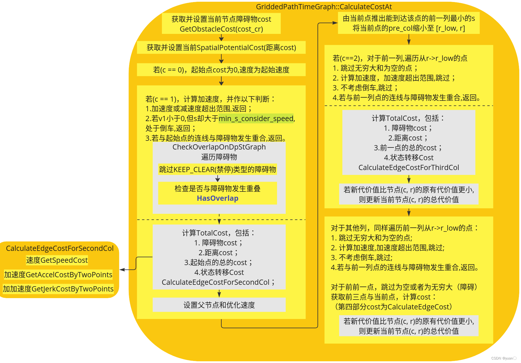
CalculateCostAt主要是计算节点的cost，对于第一列、第二列以及第三列进行特殊计算，计算之后，更新代价值。

cost主要包含四部分：

1. 障碍物的cost
2. 距离cost
3. 上一节点/起始点的cost
4. 状态转移cost

具体cost计算会在后续进行介绍

void GriddedPathTimeGraph::CalculateCostAt(const std::shared_ptr<StGraphMessage>& msg) {const uint32_t c = msg->c;const uint32_t r = msg->r;auto& cost_cr = cost_table_[c][r];// 获取并设置当前obstacle_costcost_cr.SetObstacleCost(dp_st_cost_.GetObstacleCost(cost_cr));// 当前点的障碍物代价无穷大，直接返回if (cost_cr.obstacle_cost() > std::numeric_limits<double>::max()) {return;}// 获取并设置当前SpatialPotentialCost(距离cost)cost_cr.SetSpatialPotentialCost(dp_st_cost_.GetSpatialPotentialCost(cost_cr));// 起始点cost为0，速度为起始速度const auto& cost_init = cost_table_[0][0];if (c == 0) {DCHECK_EQ(r, 0U) << "Incorrect. Row should be 0 with col = 0. row: " << r;cost_cr.SetTotalCost(0.0);cost_cr.SetOptimalSpeed(init_point_.v());return;}const double speed_limit = speed_limit_by_index_[r];const double cruise_speed = st_graph_data_.cruise_speed();// The mininal s to model as constant acceleration formula// default: 0.25 * 7 = 1.75 mconst double min_s_consider_speed = dense_unit_s_ * dimension_t_;//第2列的特殊处理if (c == 1) {// v1 = v0 + a * t, v1^2 - v0^2 = 2 * a * s => a = 2 * (s/t - v)/tconst double acc =2 * (cost_cr.point().s() / unit_t_ - init_point_.v()) / unit_t_;// 加速度或减速度超出范围，返回if (acc < max_deceleration_ || acc > max_acceleration_) {return;}// 若v1小于0，但s却大于min_s_consider_speed，倒车，返回if (init_point_.v() + acc * unit_t_ < -kDoubleEpsilon &&cost_cr.point().s() > min_s_consider_speed) {return;}// 若与起始点的连线与障碍物发生重合,返回。if (CheckOverlapOnDpStGraph(st_graph_data_.st_boundaries(), cost_cr,cost_init)) {return;}// 计算当前点的total_costcost_cr.SetTotalCost(cost_cr.obstacle_cost() + cost_cr.spatial_potential_cost() +cost_init.total_cost() +CalculateEdgeCostForSecondCol(r, speed_limit, cruise_speed));cost_cr.SetPrePoint(cost_init); //前一个点为初始点cost_cr.SetOptimalSpeed(init_point_.v() + acc * unit_t_);return;}static constexpr double kSpeedRangeBuffer = 0.20;// 估算前一点最小的sconst double pre_lowest_s =cost_cr.point().s() -FLAGS_planning_upper_speed_limit * (1 + kSpeedRangeBuffer) * unit_t_;// 找到第一个不小于pre_lowest_s的元素const auto pre_lowest_itr =std::lower_bound(spatial_distance_by_index_.begin(),spatial_distance_by_index_.end(), pre_lowest_s);uint32_t r_low = 0;// 找到r_lowif (pre_lowest_itr == spatial_distance_by_index_.end()) {r_low = dimension_s_ - 1;} else {r_low = static_cast<uint32_t>(std::distance(spatial_distance_by_index_.begin(), pre_lowest_itr));}// 由当前点推出能到达该点的前一列最小的s// 将当前点的pre_col缩小至 [r_low, r]const uint32_t r_pre_size = r - r_low + 1;const auto& pre_col = cost_table_[c - 1];double curr_speed_limit = speed_limit;// 第3列的特殊处理if (c == 2) {// 对于前一列，遍历从r->r_low的点， // 依据重新算得的cost，当前点的pre_point，也就是DP过程的状态转移方程for (uint32_t i = 0; i < r_pre_size; ++i) {uint32_t r_pre = r - i;// 跳过无穷大和为空的点if (std::isinf(pre_col[r_pre].total_cost()) ||pre_col[r_pre].pre_point() == nullptr) {continue;}// TODO(Jiaxuan): Calculate accurate acceleration by recording speed// data in ST point.// Use curr_v = (point.s - pre_point.s) / unit_t as current v// Use pre_v = (pre_point.s - prepre_point.s) / unit_t as previous v// Current acc estimate: curr_a = (curr_v - pre_v) / unit_t// = (point.s + prepre_point.s - 2 * pre_point.s) / (unit_t * unit_t)// 计算加速度const double curr_a =2 *((cost_cr.point().s() - pre_col[r_pre].point().s()) / unit_t_ -pre_col[r_pre].GetOptimalSpeed()) /unit_t_;// 加速度超出范围，跳过if (curr_a < max_deceleration_ || curr_a > max_acceleration_) {continue;}// 不考虑倒车，跳过if (pre_col[r_pre].GetOptimalSpeed() + curr_a * unit_t_ <-kDoubleEpsilon &&cost_cr.point().s() > min_s_consider_speed) {continue;}// Filter out continuous-time node connection which is in collision with// obstacle// 检查连线是否会发生碰撞if (CheckOverlapOnDpStGraph(st_graph_data_.st_boundaries(), cost_cr,pre_col[r_pre])) {continue;}curr_speed_limit =std::fmin(curr_speed_limit, speed_limit_by_index_[r_pre]);const double cost = cost_cr.obstacle_cost() +cost_cr.spatial_potential_cost() +pre_col[r_pre].total_cost() +CalculateEdgeCostForThirdCol(r, r_pre, curr_speed_limit, cruise_speed);// 若新代价值比节点（c, r）的原有代价值更小，则更新当前节点（c, r)的总代价值if (cost < cost_cr.total_cost()) {cost_cr.SetTotalCost(cost);cost_cr.SetPrePoint(pre_col[r_pre]);cost_cr.SetOptimalSpeed(pre_col[r_pre].GetOptimalSpeed() +curr_a * unit_t_);}}return;}// 其他列的处理// 依据重新算得的cost，当前点的pre_point，也就是DP过程的状态转移方程for (uint32_t i = 0; i < r_pre_size; ++i) {uint32_t r_pre = r - i;// 对于前一列，遍历从r->r_low的点， if (std::isinf(pre_col[r_pre].total_cost()) ||pre_col[r_pre].pre_point() == nullptr) {continue;}// Use curr_v = (point.s - pre_point.s) / unit_t as current v// Use pre_v = (pre_point.s - prepre_point.s) / unit_t as previous v// Current acc estimate: curr_a = (curr_v - pre_v) / unit_t// = (point.s + prepre_point.s - 2 * pre_point.s) / (unit_t * unit_t)const double curr_a =2 *((cost_cr.point().s() - pre_col[r_pre].point().s()) / unit_t_ -pre_col[r_pre].GetOptimalSpeed()) /unit_t_;if (curr_a > max_acceleration_ || curr_a < max_deceleration_) {continue;}if (pre_col[r_pre].GetOptimalSpeed() + curr_a * unit_t_ < -kDoubleEpsilon &&cost_cr.point().s() > min_s_consider_speed) {continue;}if (CheckOverlapOnDpStGraph(st_graph_data_.st_boundaries(), cost_cr,pre_col[r_pre])) {continue;}// 前前一点的rowuint32_t r_prepre = pre_col[r_pre].pre_point()->index_s();const StGraphPoint& prepre_graph_point = cost_table_[c - 2][r_prepre];// 跳过无穷大if (std::isinf(prepre_graph_point.total_cost())) {continue;}// 跳过为空的情况if (!prepre_graph_point.pre_point()) {continue;}// 前前前一点const STPoint& triple_pre_point = prepre_graph_point.pre_point()->point();// 前前一点const STPoint& prepre_point = prepre_graph_point.point();// 前一点const STPoint& pre_point = pre_col[r_pre].point();// 当前点const STPoint& curr_point = cost_cr.point();curr_speed_limit =std::fmin(curr_speed_limit, speed_limit_by_index_[r_pre]);double cost = cost_cr.obstacle_cost() + cost_cr.spatial_potential_cost() +pre_col[r_pre].total_cost() +CalculateEdgeCost(triple_pre_point, prepre_point, pre_point,curr_point, curr_speed_limit, cruise_speed);if (cost < cost_cr.total_cost()) {cost_cr.SetTotalCost(cost);cost_cr.SetPrePoint(pre_col[r_pre]);cost_cr.SetOptimalSpeed(pre_col[r_pre].GetOptimalSpeed() +curr_a * unit_t_);}}
}

2.1 GetObstacleCost障碍物cost计算

S_safe_overtake超车的安全距离
S_safe_follow跟车的安全距离

• 遍历每个障碍物ST边界，当i时刻j点恰好在障碍物边界内，说明会与障碍物发生碰撞，cost为无穷大
• 当j位置的s在障碍物上边界以上，且保留有安全超车的距离s_safe_overtake时，cost为0
• 当j在障碍物下边界以下，且保留有足够跟车安全距离s_safe_follow时，cost为0
• 其他情况则为和安全距离差值的平方乘以障碍物权重

于是整理可得：
$$C_{obs}(i,j)=\left\{\begin{array}{cc}inf，& s_{obs\cdot lower}(i)\le s(j)\le s_{obs\cdot upper}(i)\\ 0，& s(j)\ge s_{obs\cdot upper}(i)+s_{safe.overtake}\\ 0，& s(j)\le s_{obs.lower}(i)-s_{safe.follow}\\ w_{obs}[s(j)-(s_{obs.lower}(i)-s_{safe.follow}){]}^2& s_{obs.lower}(i)-s_{safe.follow}\le s(j)\le s_{obs.lower}(i)\\ w_{obs}[(s_{obs.upper}(i)+s_{safe.upper})-s(j){]}^2& s_{obs.upper}(i)\le s(j)\le s_{obs.upper}(i)+s_{safe.overtake}\end{array}\right\}$$

i是t方向上的索引，j是s方向上的索引

double DpStCost::GetObstacleCost(const StGraphPoint& st_graph_point) {const double s = st_graph_point.point().s();const double t = st_graph_point.point().t();double cost = 0.0;if (FLAGS_use_st_drivable_boundary) {// TODO(Jiancheng): move to configsstatic constexpr double boundary_resolution = 0.1;int index = static_cast<int>(t / boundary_resolution);const double lower_bound =st_drivable_boundary_.st_boundary(index).s_lower();const double upper_bound =st_drivable_boundary_.st_boundary(index).s_upper();// 在障碍物之内，无穷大if (s > upper_bound || s < lower_bound) {return kInf;}}// 遍历障碍物for (const auto* obstacle : obstacles_) {// Not applying obstacle approaching cost to virtual obstacle like created// stop fences// 跳过虚拟障碍物if (obstacle->IsVirtual()) {continue;}// Stop obstacles are assumed to have a safety margin when mapping them out,// so repelling force in dp st is not needed as it is designed to have adc// stop right at the stop distance we design in prior mapping process// 拥有STOP决策的障碍物已经留有安全空间（Speedboundsdecider），跳过if (obstacle->LongitudinalDecision().has_stop()) {continue;}auto boundary = obstacle->path_st_boundary();// FLAGS_speed_lon_decision_horizon: Longitudinal horizon for speed decision making (meter)  200.0// 跳过距离太远的障碍物if (boundary.min_s() > FLAGS_speed_lon_decision_horizon) {continue;}// 跳过不在时间范围内的障碍物if (t < boundary.min_t() || t > boundary.max_t()) {continue;}// 若与障碍物发生碰撞，cost为无穷大if (boundary.IsPointInBoundary(st_graph_point.point())) {return kInf;}double s_upper = 0.0;double s_lower = 0.0;// 获取障碍物的s_upper和s_lowerint boundary_index = boundary_map_[boundary.id()];// 障碍物逆向行驶?if (boundary_cost_[boundary_index][st_graph_point.index_t()].first < 0.0) {boundary.GetBoundarySRange(t, &s_upper, &s_lower);boundary_cost_[boundary_index][st_graph_point.index_t()] =std::make_pair(s_upper, s_lower);} else {s_upper = boundary_cost_[boundary_index][st_graph_point.index_t()].first;s_lower = boundary_cost_[boundary_index][st_graph_point.index_t()].second;}if (s < s_lower) {const double follow_distance_s = config_.safe_distance(); // safe_distance: 20.0// 在障碍物下边界以下，且保留有足够跟车安全距离follow_distance_s，cost为0if (s + follow_distance_s < s_lower) {continue;} else {auto s_diff = follow_distance_s - s_lower + s;// obstacle_weight: 1.0, default_obstacle_cost: 1e4// 用距离差值的平方进行计算cost += config_.obstacle_weight() * config_.default_obstacle_cost() *s_diff * s_diff;}} else if (s > s_upper) {const double overtake_distance_s =StGapEstimator::EstimateSafeOvertakingGap();// 在障碍物上边界以上，且保留有安全超车的距离overtake_distance_s，cost为0if (s > s_upper + overtake_distance_s) {  // or calculated from velocitycontinue;} else {auto s_diff = overtake_distance_s + s_upper - s;cost += config_.obstacle_weight() * config_.default_obstacle_cost() *s_diff * s_diff;}}}// 意味着直接continue的情况就是cost = 0return cost * unit_t_;
}

2.2 GetSpatialPotentialCost距离cost计算

目的是更快的到达目的地

距离cost计算方式如下

$$C_{spatial}=w_{spatial}(s_{total}-s(j))$$$w_{spatial}$为损失权值
$(s_{total}-s(j))$当前点到目标点的差值。

double DpStCost::GetSpatialPotentialCost(const StGraphPoint& point) {return (total_s_ - point.point().s()) * config_.spatial_potential_penalty(); // spatial_potential_penalty: 1.0e2
}

2.3 状态转移cost

这部分主要涉及三个函数：CalculateEdgeCost、CalculateEdgeCostForSecondCol以及CalculateEdgeCostForThirdCol，后两者是特殊情况，因此首先看CalculateEdgeCost。

2.3.1 CalculateEdgeCost

double GriddedPathTimeGraph::CalculateEdgeCost(const STPoint& first, const STPoint& second, const STPoint& third,const STPoint& forth, const double speed_limit, const double cruise_speed) {return dp_st_cost_.GetSpeedCost(third, forth, speed_limit, cruise_speed) +dp_st_cost_.GetAccelCostByThreePoints(second, third, forth) +dp_st_cost_.GetJerkCostByFourPoints(first, second, third, forth);
}

状态转移cost计算分为三个部分：
$$C_{edge}=C_{speed}+C_{acc}+C_{jerk}$$$C_{speed}$——速度代价
$C_{acc}$——加速度代价
$C_{jerk}$——加加速度代价

2.3.1.1 $C_{speed}$——速度代价

节点间速度为：$v=\frac{s(j)-s(j-1)}{\Delta t}$
限速比率：$v_{det}=\frac{v-v_{limit}}{v_{limit}}$
巡航速度差值：$v_{diff}=v-v_{cruise}$

$C_{speed}$速度代价的计算如下：
$$C_{speed}=\{\begin{array}{cc}inf& v<0\\ w_{KeepClear}{w}_{v-default}\Delta t& v<v_{max.adc.stop},InKeepClearRange(s(j))\\ w_{v-exceed}{w}_{v-default}(v_{det}{)}^2\Delta t& v>0,v_{det}>0\\ -w_{v-low}{w}_{v-default}{v}_{det}\Delta t& v>0,v_{det}<0\\ w_{v-ref}{w}_{v-default}|v_{diff}|\Delta t& \text{enable dp reference speed}\end{array}$$
若速度<0，则是倒车的状况，轨迹不可行，代价值设为无穷大；若速度较低且当前位置处于禁停区，则需要快速通过；若速度>0,且高于限速，则会有超速的惩罚；若速度<0,且低于限速，则会有低速的惩罚；若启用FLAGS_enable_dp_reference_speed，则会使速度靠近巡航速度。在Apollo中，超速的惩罚值（1000）远大于低速的惩罚值（10）。

double DpStCost::GetSpeedCost(const STPoint& first, const STPoint& second,const double speed_limit,const double cruise_speed) const {double cost = 0.0;const double speed = (second.s() - first.s()) / unit_t_;// 倒车的状况，轨迹不可行，代价值设为无穷大if (speed < 0) {return kInf;}// max_abs_speed_when_stopped: 0.2const double max_adc_stop_speed = common::VehicleConfigHelper::Instance()->GetConfig().vehicle_param().max_abs_speed_when_stopped();// 禁停区快速驶过if (speed < max_adc_stop_speed && InKeepClearRange(second.s())) {// first.s in range// keep_clear_low_speed_penalty: 10.0 ; default_speed_cost: 1.0e3cost += config_.keep_clear_low_speed_penalty() * unit_t_ *config_.default_speed_cost();}double det_speed = (speed - speed_limit) / speed_limit;if (det_speed > 0) {// exceed_speed_penalty: 1.0e3cost += config_.exceed_speed_penalty() * config_.default_speed_cost() *(det_speed * det_speed) * unit_t_;} else if (det_speed < 0) {// low_speed_penalty: 10.0cost += config_.low_speed_penalty() * config_.default_speed_cost() *-det_speed * unit_t_;}// True to penalize dp result towards default cruise speed// reference_speed_penalty: 10.0if (FLAGS_enable_dp_reference_speed) {double diff_speed = speed - cruise_speed;cost += config_.reference_speed_penalty() * config_.default_speed_cost() *fabs(diff_speed) * unit_t_;}return cost;
}

2.3.1.2 $C_{acc}$——加速度代价

加速度的计算如下：
$$a=\frac{s_3+s_1-2s_2}{{\Delta t}^2}$$
$C_{acc}$加速度代价的计算如下：

$$cos{t}_a=\{\begin{array}{cc}inf& a>a_{max}|a<a_{demax}\\ w_{acc}{a}^2++\frac{w_{deacc}^2{a}^2}{1+e^{a-a_{demax}}}+\frac{w_{deacc}^2{a}^2}{1+e^{-a+a_{max}}}& 0<a<a_{max}\\ w_{deacc}{a}^2+\frac{w_{deacc}^2{a}^2}{1+e^{a-a_{demax}}}+\frac{w_{deacc}^2{a}^2}{1+e^{-a+a_{max}}}& a_{min}<a<0\end{array}$$

若超过最大加速度或小于最小加速度，则代价值设为无穷大，若在之间，Apollo设计了这样的代价函数进行计算：$$y=x^2+\frac{x^2}{1+e^{x+a}}+\frac{x^2}{1+e^{x+b}}$$
其函数图像如下：
越靠近0，代价值越小；越靠近目标值，代价值越大，满足舒适性与平滑性。

2.3.1.3 $C_{jerk}$——加加速度代价

加加速度的计算方式如下：$$jerk=\frac{s_4-3s_3+3s_2-s_1}{\Delta t^3}$$

$$cos{t}_{jerk}=\{\begin{array}{cc}inf& jerk>jer{k}_{max},jerk<jer{k}_{min}\\ w_{positive,jerk}jer{k}^2\Delta t& 0<jerk<jer{k}_{max}\\ w_{negative,jerk}jer{k}^2\Delta t& jer{k}_{min}<jerk<0\end{array}$$

加加速度超过设定边界，设为无穷；若在之间，则按二次方的方式进行计算。加加速度越小越好。

接下来是两种特殊情况的计算：

2.3.2 CalculateEdgeCostForSecondCol

2.3.2.1 $C_{speed}$——速度代价

这部分一致。

2.3.2.2 $C_{acc}$——加速度代价

利用起始点的速度$v_{pre}$、当前点以及前一点（起始点）进行计算。
当前点的速度$v_{cur}=\frac{s_{cur}-s_{pre}}{\Delta t}$
加速度$a=\frac{v_{cur}-v_{pre}}{\Delta t}$
剩余部分一致。

2.3.2.3 $C_{jerk}$——加加速度代价

利用起始点的速度$v_{pre}$、起始点的加速度$a_{pre}$、当前点以及前一点（起始点）进行计算。
当前点的速度$v_{cur}=\frac{s_{cur}-s_{pre}}{\Delta t}$
当前点的加速度$a_{cur}=\frac{v_{cur}-v_{pre}}{\Delta t}$
加加速度$jerk=\frac{a_{cur}-a_{pre}}{\Delta t}$
剩余部分一致。

2.3.3 CalculateEdgeCostForThirdCol

2.3.3.1 $C_{speed}$——速度代价

这部分一致。

2.3.3.2 $C_{acc}$——加速度代价

这部分一致。

2.3.3.3 $C_{jerk}$——加加速度代价

利用起始点的速度$v_1$、当前点3、前一点2、前两点(起始点)1进行计算。
前一点速度$v_2=\frac{s_2-s_1}{\Delta t}$
前一点加速度$a_2=\frac{v_2-v_1}{\Delta t}$
当前点速度$v_3=\frac{s_3-s_2}{\Delta t}$
当前点加速度$a_3=\frac{v_3-v_2}{\Delta t}$
加加速度$jerk=\frac{a_3-a_2}{\Delta t}$
剩余部分一致。

2.4 GetRowRange

GetRowRange利用最大加速度/减速度推算下一次s(行数)的范围

void GriddedPathTimeGraph::GetRowRange(const StGraphPoint& point,size_t* next_highest_row,size_t* next_lowest_row) {double v0 = 0.0;// TODO(all): Record speed information in StGraphPoint and deprecate this.// A scaling parameter for DP range search due to the lack of accurate// information of the current velocity (set to 1 by default since we use// past 1 second's average v as approximation)double acc_coeff = 0.5;if (!point.pre_point()) {// 没有前继节点，用起始点速度代替v0 = init_point_.v();} else {// 获取当前点的速度v0 = point.GetOptimalSpeed();}const auto max_s_size = dimension_s_ - 1;const double t_squared = unit_t_ * unit_t_;// 用最大匀加速推算s的上限const double s_upper_bound = v0 * unit_t_ +acc_coeff * max_acceleration_ * t_squared +point.point().s();const auto next_highest_itr =std::lower_bound(spatial_distance_by_index_.begin(),spatial_distance_by_index_.end(), s_upper_bound);if (next_highest_itr == spatial_distance_by_index_.end()) {*next_highest_row = max_s_size;} else {*next_highest_row =std::distance(spatial_distance_by_index_.begin(), next_highest_itr);}// 用最大匀减速推算s的下限const double s_lower_bound =std::fmax(0.0, v0 * unit_t_ + acc_coeff * max_deceleration_ * t_squared) +point.point().s();const auto next_lowest_itr =std::lower_bound(spatial_distance_by_index_.begin(),spatial_distance_by_index_.end(), s_lower_bound);if (next_lowest_itr == spatial_distance_by_index_.end()) {*next_lowest_row = max_s_size;} else {*next_lowest_row =std::distance(spatial_distance_by_index_.begin(), next_lowest_itr);}
}

3. 回溯找到最优S-T曲线

需要注意回溯起点的选择

• 遍历每一列的最后一个点，找正在的best_end_point，并更新min_cost
• 这里不直接使用最后一列的min_cost点作为终点

因为采样时间是一个预估时间窗口，在这之前可能就到达终点了

Status GriddedPathTimeGraph::RetrieveSpeedProfile(SpeedData* const speed_data) {// 初始化最小代价值min_costdouble min_cost = std::numeric_limits<double>::infinity();// 初始化最优终点(即包含最小代价值的节点)const StGraphPoint* best_end_point = nullptr;// 从最后一列找到min_costfor (const StGraphPoint& cur_point : cost_table_.back()) {if (!std::isinf(cur_point.total_cost()) &&cur_point.total_cost() < min_cost) {best_end_point = &cur_point;min_cost = cur_point.total_cost();}}// 遍历每一列的最后一个点，找正在的best_end_point，并更新min_cost// 这里不直接使用最后一列的min_cost点作为终点// 因为采样时间是一个预估时间窗口，在这之前可能就到达终点了for (const auto& row : cost_table_) {const StGraphPoint& cur_point = row.back();if (!std::isinf(cur_point.total_cost()) &&cur_point.total_cost() < min_cost) {best_end_point = &cur_point;min_cost = cur_point.total_cost();}}// 寻找最优失败if (best_end_point == nullptr) {const std::string msg = "Fail to find the best feasible trajectory.";AERROR << msg;return Status(ErrorCode::PLANNING_ERROR, msg);}// 回溯，得到最优的 speed_profilestd::vector<SpeedPoint> speed_profile;const StGraphPoint* cur_point = best_end_point;while (cur_point != nullptr) {ADEBUG << "Time: " << cur_point->point().t();ADEBUG << "S: " << cur_point->point().s();ADEBUG << "V: " << cur_point->GetOptimalSpeed();SpeedPoint speed_point;speed_point.set_s(cur_point->point().s());speed_point.set_t(cur_point->point().t());speed_profile.push_back(speed_point);cur_point = cur_point->pre_point();}// 倒序std::reverse(speed_profile.begin(), speed_profile.end());static constexpr double kEpsilon = std::numeric_limits<double>::epsilon();if (speed_profile.front().t() > kEpsilon ||speed_profile.front().s() > kEpsilon) {const std::string msg = "Fail to retrieve speed profile.";AERROR << msg;return Status(ErrorCode::PLANNING_ERROR, msg);}// 计算速度for (size_t i = 0; i + 1 < speed_profile.size(); ++i) {const double v = (speed_profile[i + 1].s() - speed_profile[i].s()) /(speed_profile[i + 1].t() - speed_profile[i].t() + 1e-3);speed_profile[i].set_v(v);}*speed_data = SpeedData(speed_profile);return Status::OK();
}

最后输出为speed_data。

参考

[1] Planning 基于动态规划的速度规划
[2] Apollo 6.0的EM Planner (3)：速度规划的动态规划DP过程
[3] Apollo星火计划学习笔记——Apollo速度规划算法原理与实践
[4] 动态规划及其在Apollo项目Planning模块的应用
[5] Apollo规划控制学习笔记