论文连接：

原因

1、全部按照一个策略如IOU来分配GT和Anchors不能得到全局最优，可能只能得到局部最优。
2、目前提出的ATSS和PAA等，这些方法探索了单个对象的最佳分配策略，而未能从全局的角度考虑上下文信息。
3、目前从全局角度考虑分配信息的DeTR，采用的是匈牙利匹配算法，可以达到 one to one 的最优匹配，但是不能达到 one to many 的最优匹配。（one to many 目前来看可以加速网络训练，使得网络收敛更快）。

步骤

什么是最优传输策略

最优运输（OT）描述了以下问题：
  假设某个地区有$m$个供给者和$n$个需求者。第$i$个供应商持有$s_i$个单位的货物，而第$j$个需求者需要$d_j$个单位的货物。从供应商$i$到需求商$j$的每单位货物的运输成本由$c_{ij}$表示。
–> 我们想要找到一个运输方法，根据该方法，可以以最小的运输成本将来自供应商的所有货物运输到需求方：
$$\begin{array}{rl}\underset{\pi }{\min }& \sum _{i=1}^m\sum _{j=1}^n{c}_{ij}{\pi }_{ij}.\\ \text{ s.t. }& \sum _{i=1}^m{\pi }_{ij}=d_j,\sum _{j=1}^n{\pi }_{ij}=s_i,\\ & \sum _{i=1}^m{s}_i=\sum _{j=1}^n{d}_j,\\ & {\pi }_{ij}\ge 0,i=1,2,\dots m,j=1,2,\dots n.\end{array}$$
这是一个可以在多项式时间内求解的线性规划。然而，在我们的情况下，所得到的线性规划是大的，涉及到所有尺度的锚的特征尺寸的平方。因此，我们通过一个名为Sinkhorn-Knopp的快速迭代解来解决这个问题。

标签分配的OT

正标签分配

  在对象检测的上下文中，假设输入图像$I$有$m$个gt真实框和$n$个锚(跨越所有FPN层)，我们将每个gt视为拥有$k$个正标签单位(即$s_i=k，i=1，2，...，m$)的供应商，而每个锚作为需要一个单位标签(即$d_j=1，j=1，2，...，n$)的需求者。将一单位真实标签从$g{t}_i$运输到锚$a_j$的成本$c^{fg}$定义为其$cls$(类别损失)和$reg$(位置损失)的加权总和：
$$\begin{gathered} c_{ij}^{fg}=L_{cls}\left(P_j^{cls}(\theta ),G_i^{cls}\right)+ \\ \alpha L_{reg}\left(P_j^{box}(\theta ),G_i^{box}\right) \end{gathered}$$

其中$\theta$为模型参数。$P_j^{cls}$和$P_j^{box}$表示预测的$cls$分数和$a_j$的边界框。$G_i^{cls}$和$G_i^{box}$表示用于$g{t}_i$的真实类和边界框。$L_{cls}$和$L_{reg}$代表交叉熵损失和IoU损失。也可以用Focal Loss 和GIoU / SmoothL1 Loss 来代替这两种损失。$\alpha$为平衡系数。

负标签分配

  排除正分配之外，在训练期间会将大量锚点视为负样本。由于最佳运输涉及所有锚点，我们引入另一个供应商-背景，谁只提供负面标签。在一个标准的OT问题中，总供给必须等于总需求。因此，我们将背景可以提供的负标签的数量设置为$n-m\times k$。将一个单位的负标签从后台运输到$a_j$的成本定义为：
$$c_j^{bg}=L_{cls}(P_j^{cls}(\theta ),\varnothing ),$$
其中$\varnothing$表示背景类。将此$c^{bg}\in R^{1\times n}$与$c^{fg}\in R^{m\times n}$的最后一行连接起来，我们可以得到成本矩阵$c\in R^{(m+1)\times n}$的完全形式。供应向量s应相应地更新为：
$$s_i=\{\begin{array}{ll}k,& ifi\le m\\ n-m\times k,& ifi=m+1.\end{array}$$

损失计算

  由于我们已经有了成本矩阵$c$，供应向量$s\in R^{m+1}$，需求向量$d\in R^n$，因此可以通过现成的$Sinkhorn-Knopp迭代$来解决这个OT问题，从而获得最优运输计划${\pi }^{\ast }\in R^{(m+1)\times n}$。在得到${\pi }^{\ast }$之后，可以通过将每个锚分配给向其运输最大量的标签的供应商来解码对应的标签分配解决方案。随后的处理（例如，基于分配结果计算损耗，反向传播）与 FCOS 和 ATSS 中完全相同。注意到 OT 问题的优化过程只包含一些可以通过GPU设备加速的矩阵乘法，因此OTA只增加了不到20%的总训练时间，并且在测试阶段完全免费。

中心点距离保持稳定

  仅从具有有限区域的对象的中心区域选择正锚点，称为中心优先级。中心优先会在后续过程中存在 1、遭受大量模糊的锚点 2、或不良的统计数据。
  OTA不是依赖于统计特征，而是基于全局优化方法，因此自然可以抵抗这两个问题。理论上，OTA可以将gts框区域内的任何锚指定为正样本。然而，对于像COCO这样的一般检测数据集，我们发现中心先验仍然有利于OTA的训练。强制检测器聚焦于潜在的积极区域（即，中心区域）可以帮助稳定训练过程，特别是在训练的早期阶段，这将导致更好的最终表现。因此，我们对成本矩阵施加中心优先级。对于每个gt，我们根据锚点和gts之间的中心距离从每个FPN层上选择$r^2$个最近的锚点。对于不在$r^2$最接近列表中的锚点，它们在成本矩阵c中的对应条目将附加恒定成本，以降低它们在训练阶段期间被分配为正样本的可能性。节中4，我们将证明，虽然OTA像其他作品[38，47，48]一样采用一定程度的中心先验，但当r设置为大值时（即，大量潜在的正锚点以及更模糊的锚点）。

动态k的选取

  直观上，每个 gt 的正锚点的适当数量（即 $s_i$）应该不同，并且基于许多因素，如对象的大小、比例和遮挡条件等。因为很难直接对映射进行建模将这些因素与正锚点的数量函数联系起来，
  我们提出了一种简单但有效的方法，根据预测边界框和 gts 之间的 IoU 值粗略估计每个 gt 的正锚点的适当数量。具体来说，对于每个 gt，我们根据 IoU 值选择前 q 个预测。这些 IoU 值相加表示该 gt 的正锚点的估计数量。我们将此方法命名为动态 k 估计。
  这种估计方法基于以下直觉：某个gt的正anchor的适当数量应该与很好地回归该gt的anchor的数量正相关。

文章中对对固定 k 和动态 k 估计策略进行了详细比较。如下图：

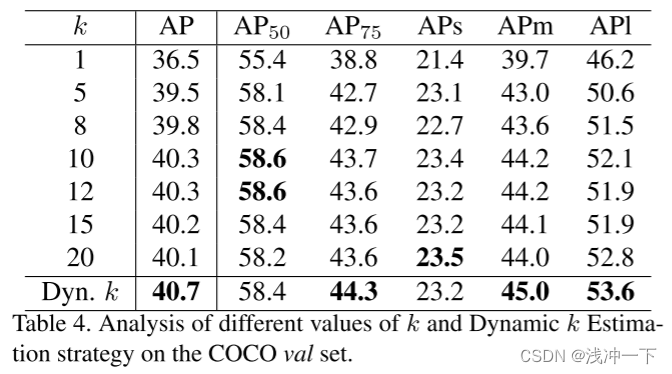
实验表明了，动态k的选取，会带来性能上的提升。

整体流程

OTA 的可视化如图 2 所示。

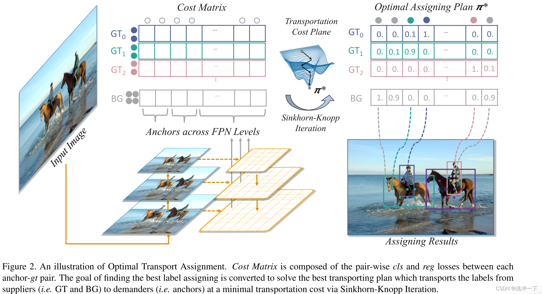
算法流程如下：
文字表述如下：

• 第一步：获得 真实框和类别。从输入数据中读取即可。
• 第二步：输入图片，得到 预测框 和 预测类别。
• 第三步：计算 真实框 和 预测框 之际的 IOU，算前面 q=20 个IOU的总和来确定每个 gt 框需要匹配的 anchor 的个数 $s_i$(被称作 dynamic k)。
• 第四步：计算 背景 需要负责的 anchor 的个数。$s_{m+1}=n-{\sum }_{i=0}^m{s}_i$。就是没有 gt 框要的那些 anchor，背景要了。
• 第五步：计算每个 gt 对所有 anchor 的 cost（包括分类 cost、回归 cost、中心点 cost）
• 第六步：优化 cost，得到最优传输方案 π*
• 第七步：每个 gt 根据前面计算得到的负责的 anchor 个数，则选择该 gt 对应的该行中，前 top-k 个位置的 anchor 作为候选框。
• 如果多个 gt 对应了一个 anchor，则在这几个 gt 中选择 cost 最小的，对该 anchor 负责。

论文流程如下：

代码

import torch.nn.functional as F
from utils.general import xywh2xyxydef box_iou(box1, box2, eps=1e-7):# https://github.com/pytorch/vision/blob/master/torchvision/ops/boxes.py"""Return intersection-over-union (Jaccard index) of boxes.Both sets of boxes are expected to be in (x1, y1, x2, y2) format.Arguments:box1 (Tensor[N, 4])box2 (Tensor[M, 4])Returns:iou (Tensor[N, M]): the NxM matrix containing the pairwiseIoU values for every element in boxes1 and boxes2"""# inter(N,M) = (rb(N,M,2) - lt(N,M,2)).clamp(0).prod(2)(a1, a2), (b1, b2) = box1.unsqueeze(1).chunk(2, 2), box2.unsqueeze(0).chunk(2, 2)inter = (torch.min(a2, b2) - torch.max(a1, b1)).clamp(0).prod(2)# IoU = inter / (area1 + area2 - inter)return inter / ((a2 - a1).prod(2) + (b2 - b1).prod(2) - inter + eps)def de_parallel(model):# De-parallelize a model: returns single-GPU model if model is of type DP or DDPreturn model.module if is_parallel(model) else modeldef xywh2xyxy(x):# Convert nx4 boxes from [x, y, w, h] to [x1, y1, x2, y2] where xy1=top-left, xy2=bottom-righty = x.clone() if isinstance(x, torch.Tensor) else np.copy(x)y[..., 0] = x[..., 0] - x[..., 2] / 2  # top left xy[..., 1] = x[..., 1] - x[..., 3] / 2  # top left yy[..., 2] = x[..., 0] + x[..., 2] / 2  # bottom right xy[..., 3] = x[..., 1] + x[..., 3] / 2  # bottom right yreturn yclass ComputeLossOTA:# Compute lossesdef __init__(self, model, autobalance=False):super(ComputeLossOTA, self).__init__()device = next(model.parameters()).device  # get model deviceh = model.hyp  # hyperparameters# Define criteriaBCEcls = nn.BCEWithLogitsLoss(pos_weight=torch.tensor([h['cls_pw']], device=device))BCEobj = nn.BCEWithLogitsLoss(pos_weight=torch.tensor([h['obj_pw']], device=device))# Class label smoothing https://arxiv.org/pdf/1902.04103.pdf eqn 3self.cp, self.cn = smooth_BCE(eps=h.get('label_smoothing', 0.0))  # positive, negative BCE targets# Focal lossg = h['fl_gamma']  # focal loss gammaif g > 0:BCEcls, BCEobj = FocalLoss(BCEcls, g), FocalLoss(BCEobj, g)det = de_parallel(model).model[-1]  # Detect() moduleself.balance = {3: [4.0, 1.0, 0.4]}.get(det.nl, [4.0, 1.0, 0.25, 0.06, .02])  # P3-P7self.ssi = list(det.stride).index(16) if autobalance else 0  # stride 16 indexself.BCEcls, self.BCEobj, self.gr, self.hyp, self.autobalance = BCEcls, BCEobj, 1.0, h, autobalancefor k in 'na', 'nc', 'nl', 'anchors', 'stride':setattr(self, k, getattr(det, k))def __call__(self, p, targets, imgs):  # predictions, targets, model   device = targets.devicelcls, lbox, lobj = torch.zeros(1, device=device), torch.zeros(1, device=device), torch.zeros(1, device=device)bs, as_, gjs, gis, targets, anchors = self.build_targets(p, targets, imgs)pre_gen_gains = [torch.tensor(pp.shape, device=device)[[3, 2, 3, 2]] for pp in p] # Lossesfor i, pi in enumerate(p):  # layer index, layer predictionsb, a, gj, gi = bs[i], as_[i], gjs[i], gis[i]  # image, anchor, gridy, gridxtobj = torch.zeros_like(pi[..., 0], device=device)  # target objn = b.shape[0]  # number of targetsif n:ps = pi[b, a, gj, gi]  # prediction subset corresponding to targets# Regressiongrid = torch.stack([gi, gj], dim=1)pxy = ps[:, :2].sigmoid() * 2. - 0.5#pxy = ps[:, :2].sigmoid() * 3. - 1.pwh = (ps[:, 2:4].sigmoid() * 2) ** 2 * anchors[i]pbox = torch.cat((pxy, pwh), 1)  # predicted boxselected_tbox = targets[i][:, 2:6] * pre_gen_gains[i]selected_tbox[:, :2] -= gridiou = bbox_iou(pbox, selected_tbox, CIoU=True)  # iou(prediction, target)if type(iou) is tuple:lbox += (iou[1].detach() * (1 - iou[0])).mean()iou = iou[0]else:lbox += (1.0 - iou).mean()  # iou loss# Objectnesstobj[b, a, gj, gi] = (1.0 - self.gr) + self.gr * iou.detach().clamp(0).type(tobj.dtype)  # iou ratio# Classificationselected_tcls = targets[i][:, 1].long()if self.nc > 1:  # cls loss (only if multiple classes)t = torch.full_like(ps[:, 5:], self.cn, device=device)  # targetst[range(n), selected_tcls] = self.cplcls += self.BCEcls(ps[:, 5:], t)  # BCE# Append targets to text file# with open('targets.txt', 'a') as file:#     [file.write('%11.5g ' * 4 % tuple(x) + '\n') for x in torch.cat((txy[i], twh[i]), 1)]obji = self.BCEobj(pi[..., 4], tobj)lobj += obji * self.balance[i]  # obj lossif self.autobalance:self.balance[i] = self.balance[i] * 0.9999 + 0.0001 / obji.detach().item()if self.autobalance:self.balance = [x / self.balance[self.ssi] for x in self.balance]lbox *= self.hyp['box']lobj *= self.hyp['obj']lcls *= self.hyp['cls']bs = tobj.shape[0]  # batch sizeloss = lbox + lobj + lclsreturn loss * bs, torch.cat((lbox, lobj, lcls)).detach()def build_targets(self, p, targets, imgs):indices, anch = self.find_3_positive(p, targets)device = torch.device(targets.device)matching_bs = [[] for pp in p]matching_as = [[] for pp in p]matching_gjs = [[] for pp in p]matching_gis = [[] for pp in p]matching_targets = [[] for pp in p]matching_anchs = [[] for pp in p]nl = len(p)    for batch_idx in range(p[0].shape[0]):b_idx = targets[:, 0]==batch_idxthis_target = targets[b_idx]if this_target.shape[0] == 0:continuetxywh = this_target[:, 2:6] * imgs[batch_idx].shape[1]txyxy = xywh2xyxy(txywh)pxyxys = []p_cls = []p_obj = []from_which_layer = []all_b = []all_a = []all_gj = []all_gi = []all_anch = []for i, pi in enumerate(p):b, a, gj, gi = indices[i]idx = (b == batch_idx)b, a, gj, gi = b[idx], a[idx], gj[idx], gi[idx]                all_b.append(b)all_a.append(a)all_gj.append(gj)all_gi.append(gi)all_anch.append(anch[i][idx])from_which_layer.append((torch.ones(size=(len(b),)) * i).to(device))fg_pred = pi[b, a, gj, gi]                p_obj.append(fg_pred[:, 4:5])p_cls.append(fg_pred[:, 5:])grid = torch.stack([gi, gj], dim=1)pxy = (fg_pred[:, :2].sigmoid() * 2. - 0.5 + grid) * self.stride[i] #/ 8.#pxy = (fg_pred[:, :2].sigmoid() * 3. - 1. + grid) * self.stride[i]pwh = (fg_pred[:, 2:4].sigmoid() * 2) ** 2 * anch[i][idx] * self.stride[i] #/ 8.pxywh = torch.cat([pxy, pwh], dim=-1)pxyxy = xywh2xyxy(pxywh)pxyxys.append(pxyxy)pxyxys = torch.cat(pxyxys, dim=0)if pxyxys.shape[0] == 0:continuep_obj = torch.cat(p_obj, dim=0)p_cls = torch.cat(p_cls, dim=0)from_which_layer = torch.cat(from_which_layer, dim=0)all_b = torch.cat(all_b, dim=0)all_a = torch.cat(all_a, dim=0)all_gj = torch.cat(all_gj, dim=0)all_gi = torch.cat(all_gi, dim=0)all_anch = torch.cat(all_anch, dim=0)pair_wise_iou = box_iou(txyxy, pxyxys)pair_wise_iou_loss = -torch.log(pair_wise_iou + 1e-8)top_k, _ = torch.topk(pair_wise_iou, min(10, pair_wise_iou.shape[1]), dim=1)dynamic_ks = torch.clamp(top_k.sum(1).int(), min=1)gt_cls_per_image = (F.one_hot(this_target[:, 1].to(torch.int64), self.nc).float().unsqueeze(1).repeat(1, pxyxys.shape[0], 1))num_gt = this_target.shape[0]cls_preds_ = (p_cls.float().unsqueeze(0).repeat(num_gt, 1, 1).sigmoid_()* p_obj.unsqueeze(0).repeat(num_gt, 1, 1).sigmoid_())y = cls_preds_.sqrt_()pair_wise_cls_loss = F.binary_cross_entropy_with_logits(torch.log(y/(1-y)) , gt_cls_per_image, reduction="none").sum(-1)del cls_preds_cost = (pair_wise_cls_loss+ 3.0 * pair_wise_iou_loss)matching_matrix = torch.zeros_like(cost, device=device)for gt_idx in range(num_gt):_, pos_idx = torch.topk(cost[gt_idx], k=dynamic_ks[gt_idx].item(), largest=False)matching_matrix[gt_idx][pos_idx] = 1.0del top_k, dynamic_ksanchor_matching_gt = matching_matrix.sum(0)if (anchor_matching_gt > 1).sum() > 0:_, cost_argmin = torch.min(cost[:, anchor_matching_gt > 1], dim=0)matching_matrix[:, anchor_matching_gt > 1] *= 0.0matching_matrix[cost_argmin, anchor_matching_gt > 1] = 1.0fg_mask_inboxes = (matching_matrix.sum(0) > 0.0).to(device)matched_gt_inds = matching_matrix[:, fg_mask_inboxes].argmax(0)from_which_layer = from_which_layer[fg_mask_inboxes]all_b = all_b[fg_mask_inboxes]all_a = all_a[fg_mask_inboxes]all_gj = all_gj[fg_mask_inboxes]all_gi = all_gi[fg_mask_inboxes]all_anch = all_anch[fg_mask_inboxes]this_target = this_target[matched_gt_inds]for i in range(nl):layer_idx = from_which_layer == imatching_bs[i].append(all_b[layer_idx])matching_as[i].append(all_a[layer_idx])matching_gjs[i].append(all_gj[layer_idx])matching_gis[i].append(all_gi[layer_idx])matching_targets[i].append(this_target[layer_idx])matching_anchs[i].append(all_anch[layer_idx])for i in range(nl):if matching_targets[i] != []:matching_bs[i] = torch.cat(matching_bs[i], dim=0)matching_as[i] = torch.cat(matching_as[i], dim=0)matching_gjs[i] = torch.cat(matching_gjs[i], dim=0)matching_gis[i] = torch.cat(matching_gis[i], dim=0)matching_targets[i] = torch.cat(matching_targets[i], dim=0)matching_anchs[i] = torch.cat(matching_anchs[i], dim=0)else:matching_bs[i] = torch.tensor([], device='cuda:0', dtype=torch.int64)matching_as[i] = torch.tensor([], device='cuda:0', dtype=torch.int64)matching_gjs[i] = torch.tensor([], device='cuda:0', dtype=torch.int64)matching_gis[i] = torch.tensor([], device='cuda:0', dtype=torch.int64)matching_targets[i] = torch.tensor([], device='cuda:0', dtype=torch.int64)matching_anchs[i] = torch.tensor([], device='cuda:0', dtype=torch.int64)return matching_bs, matching_as, matching_gjs, matching_gis, matching_targets, matching_anchs           def find_3_positive(self, p, targets):# Build targets for compute_loss(), input targets(image,class,x,y,w,h)na, nt = self.na, targets.shape[0]  # number of anchors, targetsindices, anch = [], []gain = torch.ones(7, device=targets.device).long()  # normalized to gridspace gainai = torch.arange(na, device=targets.device).float().view(na, 1).repeat(1, nt)  # same as .repeat_interleave(nt)targets = torch.cat((targets.repeat(na, 1, 1), ai[:, :, None]), 2)  # append anchor indicesg = 0.5  # biasoff = torch.tensor([[0, 0],[1, 0], [0, 1], [-1, 0], [0, -1],  # j,k,l,m# [1, 1], [1, -1], [-1, 1], [-1, -1],  # jk,jm,lk,lm], device=targets.device).float() * g  # offsetsfor i in range(self.nl):anchors = self.anchors[i]gain[2:6] = torch.tensor(p[i].shape)[[3, 2, 3, 2]]  # xyxy gain# Match targets to anchorst = targets * gainif nt:# Matchesr = t[:, :, 4:6] / anchors[:, None]  # wh ratioj = torch.max(r, 1. / r).max(2)[0] < self.hyp['anchor_t']  # compare# j = wh_iou(anchors, t[:, 4:6]) > model.hyp['iou_t']  # iou(3,n)=wh_iou(anchors(3,2), gwh(n,2))t = t[j]  # filter# Offsetsgxy = t[:, 2:4]  # grid xygxi = gain[[2, 3]] - gxy  # inversej, k = ((gxy % 1. < g) & (gxy > 1.)).Tl, m = ((gxi % 1. < g) & (gxi > 1.)).Tj = torch.stack((torch.ones_like(j), j, k, l, m))t = t.repeat((5, 1, 1))[j]offsets = (torch.zeros_like(gxy)[None] + off[:, None])[j]else:t = targets[0]offsets = 0# Defineb, c = t[:, :2].long().T  # image, classgxy = t[:, 2:4]  # grid xygwh = t[:, 4:6]  # grid whgij = (gxy - offsets).long()gi, gj = gij.T  # grid xy indices# Appenda = t[:, 6].long()  # anchor indicesindices.append((b, a, gj.clamp_(0, gain[3] - 1), gi.clamp_(0, gain[2] - 1)))  # image, anchor, grid indicesanch.append(anchors[a])  # anchorsreturn indices, anch

大神仓库：连接。、
大神CSDN：连接。

使用

在yolov5 7.0 版本中，训练 coco 数据，采用了预训练权重，采用的命令行如下：

python train.py --data coco.yaml --weights yolov5s.pt --img 640 --batch-size 32

训练过程如下：

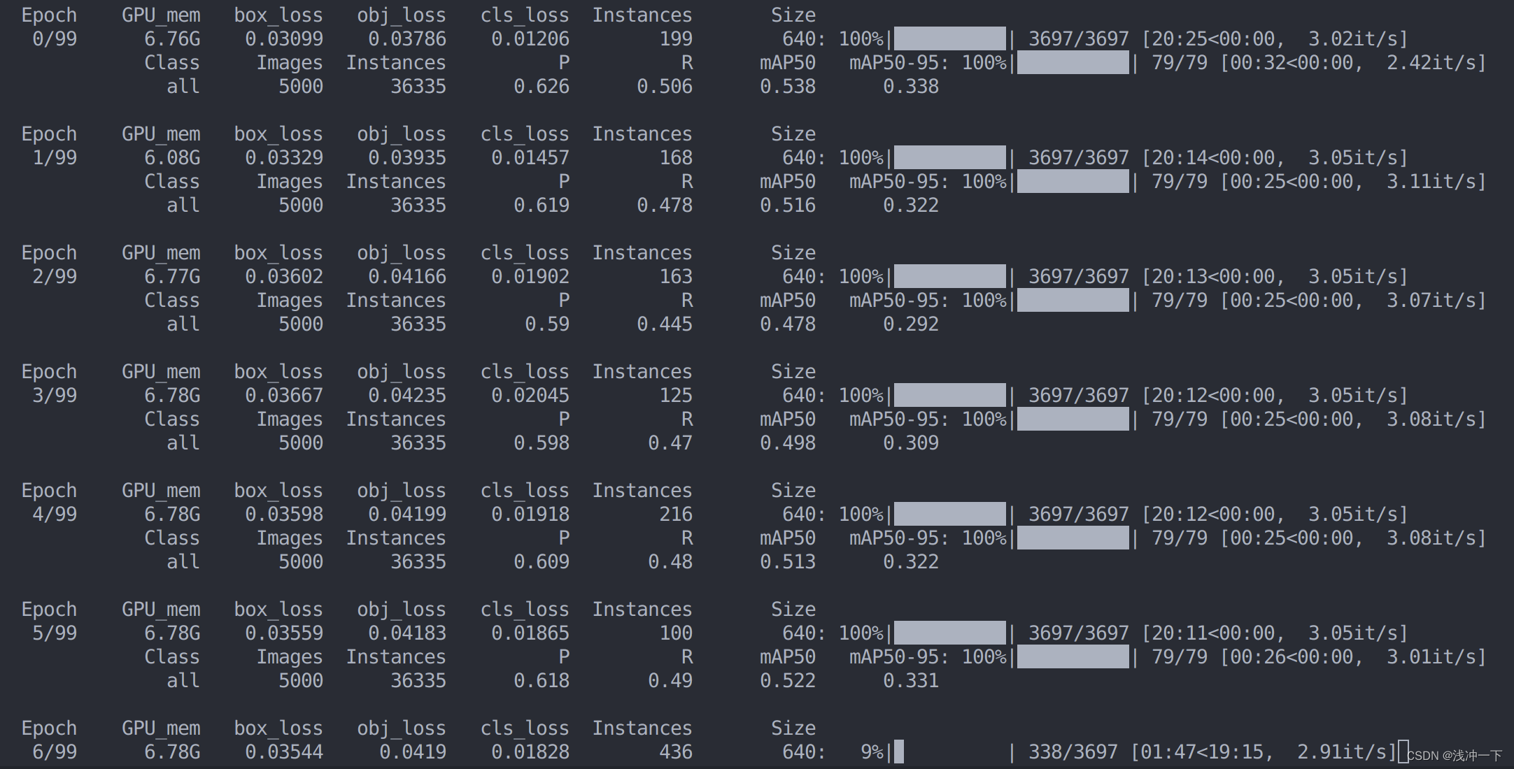
目前来看 loss 呈现，先上升再下降的趋势。等训练完 100 epoch 来再比较一下。