目录
一、数据及分析对象
二、目的及分析任务
三、方法及工具
四、数据读入
五、数据理解
六、数据准备
七、模型训练
八、模型评价
九、模型调参
十、模型预测
一、数据及分析对象
CSV文件——“bc_data.csv”
数据集链接:https://download.csdn.net/download/m0_70452407/88524905
该数据集主要记录了569个病例的32个属性,主要属性/字段如下:
(1)ID:病例的ID。
(2)Diagnosis(诊断结果):M为恶性,B为良性。该数据集共包含357个良性病例和212个恶性病例。
(3)细胞核的10个特征值,包括radius(半径)、texture(纹理)、perimeter(周长)、面积(area)、平滑度(smoothness)、紧凑度(compactness)、凹面(concavity)、凹点(concave points)、对称性(symmetry)和分形维数(fractal dimension)等。同时,为上述10个特征值分别提供了3种统计量,分别为均值(mean)、标准差(standard error)和最大值(worst or largest)。
二、目的及分析任务
理解机器学习方法在数据分析中的应用——采用逻辑回归方法进行分类分析。
(1)数据读入。
(2)划分训练集和数据集,利用逻辑回归算法进行模型训练,分类分析。
(3)进行模型评价,调整模型参数。
(4)将调参后的模型进行模型预测,得出的结果与测试集结果进行对比分析,验证逻辑回归算法建模的有效性。
三、方法及工具
Python语言及scikit-learn包。
四、数据读入
导入所需的工具包:
import pandas as pd
import numpy as np
from sklearn.linear_model import LogisticRegression
from sklearn import metrics
导入scikit-learn自带的数据集——威斯康星州乳腺癌数据集,这里采用的实现方式为调用sklearn.datasets中的load_breast_cancer()方法。
#数据读入
from sklearn.datasets import load_breast_cancer
breast_cancer=load_breast_cancer()
导入的威斯康星州乳腺癌数据集是字典数据,显示其字典的键为:
#显示数据集字典的键
print(breast_cancer.keys())
dict_keys(['data', 'target', 'frame', 'target_names', 'DESCR', 'feature_names', 'filename', 'data_module'])
输出结果中,'target'为分类目标,'DESCR'为数据集的完整性描述,'feature_names'为特征名称。
显示数据集的完整描述:
print(breast_cancer.DESCR).. _breast_cancer_dataset:Breast cancer wisconsin (diagnostic) dataset --------------------------------------------**Data Set Characteristics:**:Number of Instances: 569:Number of Attributes: 30 numeric, predictive attributes and the class:Attribute Information:- radius (mean of distances from center to points on the perimeter)- texture (standard deviation of gray-scale values)- perimeter- area- smoothness (local variation in radius lengths)- compactness (perimeter^2 / area - 1.0)- concavity (severity of concave portions of the contour)- concave points (number of concave portions of the contour)- symmetry- fractal dimension ("coastline approximation" - 1)The mean, standard error, and "worst" or largest (mean of the threeworst/largest values) of these features were computed for each image,resulting in 30 features. For instance, field 0 is Mean Radius, field10 is Radius SE, field 20 is Worst Radius.- class:- WDBC-Malignant- WDBC-Benign:Summary Statistics:===================================== ====== ======Min Max===================================== ====== ======radius (mean): 6.981 28.11texture (mean): 9.71 39.28perimeter (mean): 43.79 188.5area (mean): 143.5 2501.0smoothness (mean): 0.053 0.163compactness (mean): 0.019 0.345concavity (mean): 0.0 0.427concave points (mean): 0.0 0.201symmetry (mean): 0.106 0.304fractal dimension (mean): 0.05 0.097radius (standard error): 0.112 2.873texture (standard error): 0.36 4.885perimeter (standard error): 0.757 21.98area (standard error): 6.802 542.2smoothness (standard error): 0.002 0.031compactness (standard error): 0.002 0.135concavity (standard error): 0.0 0.396concave points (standard error): 0.0 0.053symmetry (standard error): 0.008 0.079fractal dimension (standard error): 0.001 0.03radius (worst): 7.93 36.04texture (worst): 12.02 49.54perimeter (worst): 50.41 251.2area (worst): 185.2 4254.0smoothness (worst): 0.071 0.223compactness (worst): 0.027 1.058concavity (worst): 0.0 1.252concave points (worst): 0.0 0.291symmetry (worst): 0.156 0.664fractal dimension (worst): 0.055 0.208===================================== ====== ======:Missing Attribute Values: None:Class Distribution: 212 - Malignant, 357 - Benign:Creator: Dr. William H. Wolberg, W. Nick Street, Olvi L. Mangasarian:Donor: Nick Street:Date: November, 1995This is a copy of UCI ML Breast Cancer Wisconsin (Diagnostic) datasets. https://goo.gl/U2Uwz2Features are computed from a digitized image of a fine needle aspirate (FNA) of a breast mass. They describe characteristics of the cell nuclei present in the image.Separating plane described above was obtained using Multisurface Method-Tree (MSM-T) [K. P. Bennett, "Decision Tree Construction Via Linear Programming." Proceedings of the 4th Midwest Artificial Intelligence and Cognitive Science Society, pp. 97-101, 1992], a classification method which uses linear programming to construct a decision tree. Relevant features were selected using an exhaustive search in the space of 1-4 features and 1-3 separating planes.The actual linear program used to obtain the separating plane in the 3-dimensional space is that described in: [K. P. Bennett and O. L. Mangasarian: "Robust Linear Programming Discrimination of Two Linearly Inseparable Sets", Optimization Methods and Software 1, 1992, 23-34].This database is also available through the UW CS ftp server:ftp ftp.cs.wisc.edu cd math-prog/cpo-dataset/machine-learn/WDBC/.. topic:: References- W.N. Street, W.H. Wolberg and O.L. Mangasarian. Nuclear feature extraction for breast tumor diagnosis. IS&T/SPIE 1993 International Symposium on Electronic Imaging: Science and Technology, volume 1905, pages 861-870,San Jose, CA, 1993.- O.L. Mangasarian, W.N. Street and W.H. Wolberg. Breast cancer diagnosis and prognosis via linear programming. Operations Research, 43(4), pages 570-577, July-August 1995.- W.H. Wolberg, W.N. Street, and O.L. Mangasarian. Machine learning techniquesto diagnose breast cancer from fine-needle aspirates. Cancer Letters 77 (1994) 163-171.
显示数据集的特征名称:
#数据集的特征名称
print(breast_cancer.feature_names)
['mean radius' 'mean texture' 'mean perimeter' 'mean area''mean smoothness' 'mean compactness' 'mean concavity''mean concave points' 'mean symmetry' 'mean fractal dimension''radius error' 'texture error' 'perimeter error' 'area error''smoothness error' 'compactness error' 'concavity error''concave points error' 'symmetry error' 'fractal dimension error''worst radius' 'worst texture' 'worst perimeter' 'worst area''worst smoothness' 'worst compactness' 'worst concavity''worst concave points' 'worst symmetry' 'worst fractal dimension']
显示数据形状:
#数据形状
print(breast_cancer.data.shape)
(569, 30)
调用pandas包数据框(DataFrame),将数据(data)与回归目标(target)转化为数据框类型。
#将数据(data)与回归目标(target)转换为数据框类型
X=pd.DataFrame(breast_cancer.data,columns=breast_cancer.feature_names)
y=pd.DataFrame(breast_cancer.target,columns=['class'])
将X,y数据框合并后,生成数据集df
#合并数据框
df=pd.concat([X,y],axis=1)
df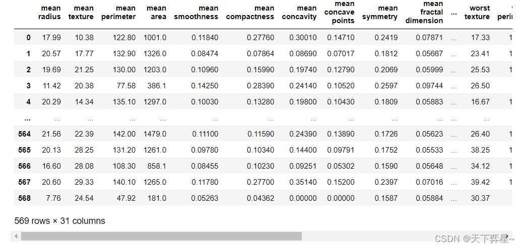
五、数据理解
查看数据基本信息:
#查看数据基本信息
df.info()
<class 'pandas.core.frame.DataFrame'> RangeIndex: 569 entries, 0 to 568 Data columns (total 31 columns):# Column Non-Null Count Dtype --- ------ -------------- ----- 0 mean radius 569 non-null float641 mean texture 569 non-null float642 mean perimeter 569 non-null float643 mean area 569 non-null float644 mean smoothness 569 non-null float645 mean compactness 569 non-null float646 mean concavity 569 non-null float647 mean concave points 569 non-null float648 mean symmetry 569 non-null float649 mean fractal dimension 569 non-null float6410 radius error 569 non-null float6411 texture error 569 non-null float6412 perimeter error 569 non-null float6413 area error 569 non-null float6414 smoothness error 569 non-null float6415 compactness error 569 non-null float6416 concavity error 569 non-null float6417 concave points error 569 non-null float6418 symmetry error 569 non-null float6419 fractal dimension error 569 non-null float6420 worst radius 569 non-null float6421 worst texture 569 non-null float6422 worst perimeter 569 non-null float6423 worst area 569 non-null float6424 worst smoothness 569 non-null float6425 worst compactness 569 non-null float6426 worst concavity 569 non-null float6427 worst concave points 569 non-null float6428 worst symmetry 569 non-null float6429 worst fractal dimension 569 non-null float6430 class 569 non-null int32 dtypes: float64(30), int32(1) memory usage: 135.7 KB
查看描述性统计信息:
#查看描述新统计信息
df.describe()
六、数据准备
利用sklearn.model_selection的train_test_split()方法划分训练集和测试集,固定random_state为42,用30%的数据测试,70%的数据训练。
#划分训练集和测试集
from sklearn.model_selection import train_test_split
X_train,X_test,y_train,y_test=train_test_split(X,y,test_size=0.3,random_state=42)
X_test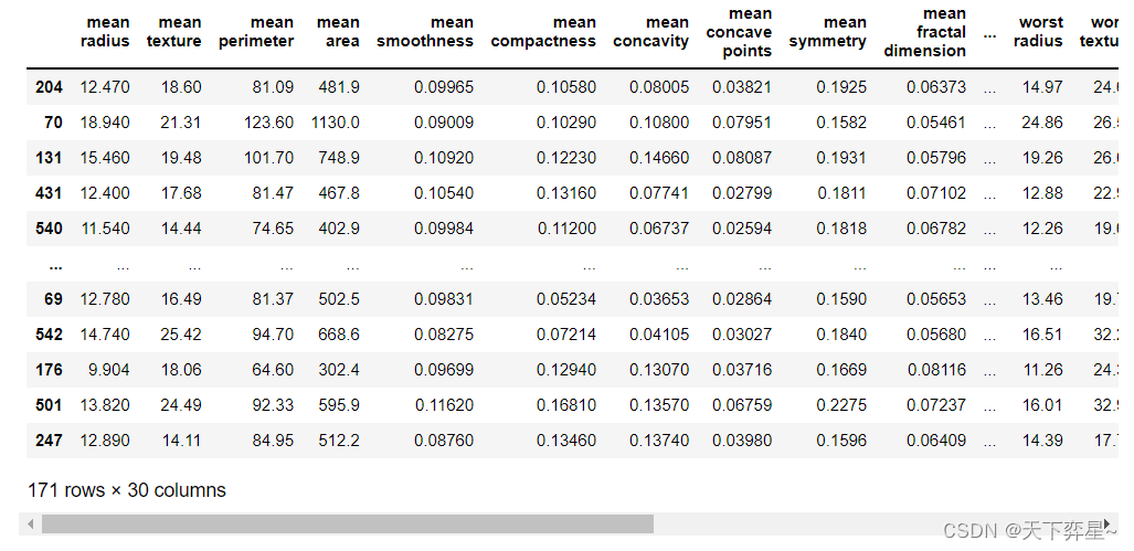
七、模型训练
调用默认参数的LogisticRegression在训练集上进行模型训练。
#模型训练
model=LogisticRegression(C=1.0,class_weight=None,dual=False,fit_intercept=True,intercept_scaling=1,max_iter=100,multi_class='ovr',n_jobs=1,penalty='l2',random_state=None,solver='liblinear',tol=0.0001,verbose=0,warm_start=False)
model.fit(X_train,y_train)
LogisticRegression(multi_class='ovr', n_jobs=1, solver='liblinear')
该输出结果显示了模型的训练结果。选择逻辑回归模型参数的默认值进行训练。选择L2正则项,C=1.0控制正则化的强度。"fit_intercept=True,intercept_scaling=1"表示增加截距缩放,减少正则化对综合特征权重的影响。"class_weight=None"表示所有类都有权重。"solver=liblinear"时(在最优化问题时使用"liblinear"算法)。max_iter=100表示求解器收敛所采用的最大迭代次数为100。multi_class="ovr"表示每个标签都适合一个二进制问题。n_jobs表示在类上并行时使用的CPU核心数量。当warm_start设置为True时,重用前一个调用的解决方案以适应初始化,否则,只需删除前一个解决方案。
显示预测结果:
#默认参数模型预测结果y_pred
y_pred=model.predict(X_test)
y_pred
array([1, 0, 0, 1, 1, 0, 0, 0, 1, 1, 1, 0, 1, 0, 1, 0, 1, 1, 1, 0, 1, 1,0, 1, 1, 1, 1, 1, 1, 0, 1, 1, 1, 1, 1, 1, 0, 1, 0, 1, 1, 0, 1, 1,1, 1, 1, 1, 1, 1, 0, 0, 1, 1, 1, 1, 1, 0, 1, 1, 1, 0, 0, 1, 1, 1,0, 0, 1, 1, 0, 0, 1, 0, 1, 1, 1, 1, 1, 1, 0, 1, 1, 0, 0, 0, 0, 0,1, 1, 1, 1, 1, 1, 1, 1, 0, 0, 1, 0, 0, 1, 0, 0, 1, 1, 1, 0, 1, 1,0, 1, 0, 0, 1, 0, 1, 1, 1, 0, 0, 1, 1, 0, 1, 0, 0, 1, 1, 0, 0, 0,1, 1, 1, 0, 1, 1, 1, 0, 1, 0, 1, 1, 0, 1, 0, 0, 0, 1, 0, 1, 1, 1,1, 0, 0, 1, 1, 1, 1, 1, 1, 1, 0, 1, 1, 1, 1, 0, 1])
八、模型评价
利用混淆矩阵分类算法的指标进行模型的分类效果评价。
#混淆矩阵(分类算法的重要评估指标)
matrix=metrics.confusion_matrix(y_test,y_pred)
matrix
array([[ 59, 4],[ 2, 106]], dtype=int64)
利用准确度(Accuracy)、精度(Precision)这两项分类指标进行模型的分类效果评价。
#分类评价指标——准确度(Accuracy)
print("Accuracy:",metrics.accuracy_score(y_test,y_pred))#分类评价指标——精度(Precision)
print("Precision:",metrics.precision_score(y_test,y_pred))
Accuracy: 0.9649122807017544 Precision: 0.9636363636363636
九、模型调参
设置GridSearchCV函数的param_grid、cv参数值。为了防止过拟合现象的出现,通过参数C控制正则化程度,C值越大,正则化越弱。一般情况下,C增大(正则化程度弱),模型的准确性在训练集和测试集上都在提升(对损失函数的惩罚减弱),特征维度更多,学习能力更强,过拟合的风险也更高。L1和L2两项正则化项对目标函数的影响不同,选择的求解模型惨啊书的梯度下降法也不同。
#以C、penalty参数和值设置字典列表param_grid。
#设置cv参数值为5
param_grid={'C':[0.001,0.01,0.1,1,10,20,50,100],'penalty':["l1","l2"]}
n_folds=5
调用GridSearchCV函数,进行5折交叉验证,得出模型最优参数:
#调用GridSearchCV函数,进行5折交叉验证,对估计器LogisticRegression()的指定参数值param_grid进行详尽搜索,得到最终的最优模型参数
from sklearn.model_selection import GridSearchCV
estimator=GridSearchCV(LogisticRegression(solver='liblinear'),param_grid,cv=n_folds)
estimator.fit(X_train,y_train)
GridSearchCV(cv=5, estimator=LogisticRegression(solver='liblinear'),param_grid={'C': [0.001, 0.01, 0.1, 1, 10, 20, 50, 100],'penalty': ['l1', 'l2']})
该输出结果显示了调用GridSearchCV()方法对估计器的指定参数值进行详尽搜索。
利用best_estimator_属性,得到通过搜索选择的最高分(或最小损失的估计量):
estimator.best_estimator_LogisticRegression(C=50, penalty='l1', solver='liblinear')
该输出结果显示了最优的模型参数为C=50,penalty="l1"
十、模型预测
调参后的模型训练:
#调参后的模型训练
model1=LogisticRegression(C=50,class_weight=None,dual=False,fit_intercept=True,intercept_scaling=1,max_iter=100,multi_class='ovr',n_jobs=1,penalty='l1',random_state=None,solver='liblinear',tol=0.0001,verbose=0,warm_start=False)
model1.fit(X_train,y_train)
LogisticRegression(C=50, multi_class='ovr', n_jobs=1, penalty='l1',solver='liblinear')
调参后的模型预测:
#调参后的模型预测
y_pred1=model1.predict(X_test)
y_pred1
array([1, 0, 0, 1, 1, 0, 0, 0, 1, 1, 1, 0, 1, 0, 1, 0, 1, 1, 1, 0, 1, 1,0, 1, 1, 1, 1, 1, 1, 0, 1, 1, 1, 1, 1, 1, 0, 1, 0, 1, 1, 0, 1, 1,1, 1, 1, 1, 1, 1, 0, 0, 1, 1, 1, 1, 1, 0, 0, 1, 1, 0, 0, 1, 1, 1,0, 0, 1, 1, 0, 0, 1, 0, 1, 1, 1, 0, 1, 1, 0, 1, 0, 0, 0, 0, 0, 0,1, 1, 1, 1, 1, 1, 1, 1, 0, 0, 1, 0, 0, 1, 0, 0, 1, 1, 1, 0, 1, 1,0, 1, 0, 0, 0, 0, 1, 1, 1, 0, 0, 1, 1, 0, 1, 0, 0, 1, 1, 0, 0, 0,1, 1, 1, 0, 1, 1, 1, 0, 1, 0, 1, 1, 0, 1, 0, 0, 0, 1, 0, 1, 1, 1,1, 0, 0, 1, 1, 1, 1, 1, 1, 1, 0, 1, 1, 1, 1, 0, 1])
调参后的模型混淆矩阵结果:
#调参后的模型混淆矩阵结果
matrix1=metrics.confusion_matrix(y_test,y_pred1)
matrix1
array([[ 62, 1],[ 3, 105]], dtype=int64)
调参后的模型准确度、精度分类指标评价结果:
#调参后的额模型准确度、精度分类指标评价结果
print("Accuracy1:",metrics.accuracy_score(y_test,y_pred1))
print("Precision1:",metrics.precision_score(y_test,y_pred1))
Accuracy1: 0.9766081871345029 Precision1: 0.9905660377358491
该输出结果显示了调参后的模型分类指标准确度(Accuracy)、精度(Precision)分类指标值。通过与之前未调参的模型分类效果进行对比,可以发现准确度(Accuracy)、精度(Precision)值提升,混淆矩阵得出的结果也更好,分类效果显著提升。