2 时间序列预测入门：GRU-编程知识

0 论文地址

GRU 原论文：https://arxiv.org/pdf/1406.1078v3.pdf

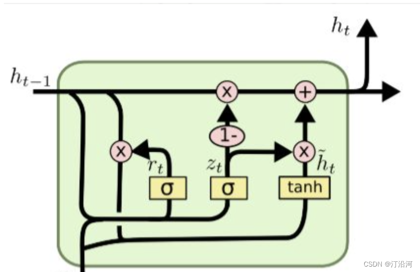
GRU（Gate Recurrent Unit）是循环神经网络（RNN）的一种，可以解决RNN中不能长期记忆和反向传播中的梯度等问题，与LSTM的作用类似，不过比LSTM简单，容易进行训练。

重置门决定了如何将新的输入信息与前面的记忆相结合。

更新门用于控制前一时刻的状态信息被带入到当前状态中的程度，也就是更新门帮助模型决定到底要将多少过去的信息传递到未来，简单来说就是用于更新记忆。

y = GRU(x,ho) 两个输入： x, h0;

需要数据的同学，也可私聊：

1 数据

数据： 2023“SEED”第四届江苏大数据开发与应用大赛--新能源赛道的数据

MARS开发者生态社区

解题思路：总共500个充电站状，关联地理位置，然后提取18个特征；把这18个特征作为时步不长（记得是某个比赛的思路）然后特征长度为1 （类比词向量的size)

data = （batch_size, time_stamp, 1 ）

其中： time_stamp对应了特征；也可以把历史特征作为训练数据的一部分，但是如何很长的序列预测如何处理值得考虑下；

1.1 单向的GRU

import numpy as np
import pandas as pd
import torch
import torch.nn as nn
#import tushare as ts
from sklearn.preprocessing import StandardScaler, MinMaxScaler
from torch.utils.data import TensorDataset
from tqdm import tqdm
from sklearn.model_selection import train_test_splitimport matplotlib.pyplot as plt
import tqdm
import sys
import os
import gc
import argparse
import warningswarnings.filterwarnings('ignore')# 读取数据
train_power_forecast_history = pd.read_csv('../data/data1/train/power_forecast_history.csv')
train_power = pd.read_csv('../data/data1/train/power.csv')
train_stub_info = pd.read_csv('../data/data1/train/stub_info.csv')test_power_forecast_history = pd.read_csv('../data/data1/test/power_forecast_history.csv')
test_stub_info = pd.read_csv('../data/data1/test/stub_info.csv')# 聚合数据
train_df = train_power_forecast_history.groupby(['id_encode','ds']).head(1)
del train_df['hour']test_df = test_power_forecast_history.groupby(['id_encode','ds']).head(1)
del test_df['hour']tmp_df = train_power.groupby(['id_encode','ds'])['power'].sum()
tmp_df.columns = ['id_encode','ds','power']# 合并充电量数据
train_df = train_df.merge(tmp_df, on=['id_encode','ds'], how='left')### 合并数据
train_df = train_df.merge(train_stub_info, on='id_encode', how='left')
test_df = test_df.merge(test_stub_info, on='id_encode', how='left')h3_code = pd.read_csv("../data/h3_lon_lat.csv")
train_df = train_df.merge(h3_code,on='h3')
test_df = test_df.merge(h3_code,on='h3')def kalman_filter(data, q=0.0001, r=0.01):# 后验初始值x0 = data[0]                              # 令第一个估计值，为当前值p0 = 1.0# 存结果的列表x = [x0]for z in data[1:]:                        # kalman 滤波实时计算，只要知道当前值z就能计算出估计值(后验值)x0# 先验值x1_minus = x0                         # X(k|k-1) = AX(k-1|k-1) + BU(k) + W(k), A=1,BU(k) = 0p1_minus = p0 + q                     # P(k|k-1) = AP(k-1|k-1)A' + Q(k), A=1# 更新K和后验值k1 = p1_minus / (p1_minus + r)        # Kg(k)=P(k|k-1)H'/[HP(k|k-1)H' + R], H=1x0 = x1_minus + k1 * (z - x1_minus)   # X(k|k) = X(k|k-1) + Kg(k)[Z(k) - HX(k|k-1)], H=1p0 = (1 - k1) * p1_minus              # P(k|k) = (1 - Kg(k)H)P(k|k-1), H=1x.append(x0)                          # 由输入的当前值z 得到估计值x0存入列表中，并开始循环到下一个值return x#kalman_filter()
train_df['new_label'] = 0
for i in range(500):#print(i)label = i#train_df[train_df['id_encode']==labe]['power'].valuestrain_df.loc[train_df['id_encode']==label, 'new_label'] = kalman_filter(data=train_df[train_df['id_encode']==label]['power'].values)### 数据预处理
train_df['flag'] = train_df['flag'].map({'A':0,'B':1})
test_df['flag'] = test_df['flag'].map({'A':0,'B':1})def get_time_feature(df, col):df_copy = df.copy()prefix = col + "_"df_copy['new_'+col] = df_copy[col].astype(str)col = 'new_'+coldf_copy[col] = pd.to_datetime(df_copy[col], format='%Y%m%d')#df_copy[prefix + 'year'] = df_copy[col].dt.yeardf_copy[prefix + 'month'] = df_copy[col].dt.monthdf_copy[prefix + 'day'] = df_copy[col].dt.day# df_copy[prefix + 'weekofyear'] = df_copy[col].dt.weekofyeardf_copy[prefix + 'dayofweek'] = df_copy[col].dt.dayofweek# df_copy[prefix + 'is_wknd'] = df_copy[col].dt.dayofweek // 6df_copy[prefix + 'quarter'] = df_copy[col].dt.quarter# df_copy[prefix + 'is_month_start'] = df_copy[col].dt.is_month_start.astype(int)# df_copy[prefix + 'is_month_end'] = df_copy[col].dt.is_month_end.astype(int)del df_copy[col]return df_copytrain_df = get_time_feature(train_df, 'ds')
test_df = get_time_feature(test_df, 'ds')train_df = train_df.fillna(999)
test_df = test_df.fillna(999)cols = [f for f in train_df.columns if f not in ['ds','power','h3','new_label']]scaler = MinMaxScaler(feature_range=(0,1))
scalar_falg = False
if scalar_falg == True:df_for_training_scaled = scaler.fit_transform(train_df[cols])df_for_testing_scaled= scaler.transform(test_df[cols])
else:df_for_training_scaled = train_df[cols]df_for_testing_scaled = test_df[cols]
#df_for_training_scaled
# scaler_label = MinMaxScaler(feature_range=(0,1))
# label_for_training_scaled = scaler_label.fit_transform(train_df['new_label']..values)
# label_for_testing_scaled= scaler_label.transform(train_df['new_label'].values)
# #df_for_training_scaledclass Config():data_path = '../data/data1/train/power.csv'timestep = 18  # 时间步长，就是利用多少时间窗口batch_size = 32  # 批次大小feature_size = 1  # 每个步长对应的特征数量，这里只使用1维，每天的风速hidden_size = 256  # 隐层大小output_size = 1  # 由于是单输出任务，最终输出层大小为1，预测未来1天风速num_layers = 2  # lstm的层数epochs = 10 # 迭代轮数best_loss = 0 # 记录损失learning_rate = 0.00003 # 学习率model_name = 'lstm' # 模型名称save_path = './{}.pth'.format(model_name) # 最优模型保存路径config = Config()x_train, x_test, y_train, y_test = train_test_split(df_for_training_scaled.values, train_df['new_label'].values,shuffle=False, test_size=0.2)# 将数据转为tensor
x_train_tensor = torch.from_numpy(x_train.reshape(-1,config.timestep,1)).to(torch.float32)
y_train_tensor = torch.from_numpy(y_train.reshape(-1,1)).to(torch.float32)
x_test_tensor = torch.from_numpy(x_test.reshape(-1,config.timestep,1)).to(torch.float32)
y_test_tensor = torch.from_numpy(y_test.reshape(-1,1)).to(torch.float32)# 5.形成训练数据集
train_data = TensorDataset(x_train_tensor, y_train_tensor)
test_data = TensorDataset(x_test_tensor, y_test_tensor)# 6.将数据加载成迭代器
train_loader = torch.utils.data.DataLoader(train_data,config.batch_size,False)test_loader = torch.utils.data.DataLoader(test_data,config.batch_size,False)#train_df[cols]
# 7.定义GRU网络
#train_df[cols]
# 7.定义LSTM网络
#train_df[cols]
# 7.定义LSTM网络
class GRUModel(nn.Module):def __init__(self, feature_size, hidden_size, num_layers, output_size):super(GRUModel, self).__init__()self.hidden_size = hidden_size  # 隐层大小self.num_layers = num_layers  # lstm层数# feature_size为特征维度，就是每个时间点对应的特征数量，这里为1self.gru = nn.GRU(feature_size, hidden_size, num_layers, batch_first=True)self.fc = nn.Linear(hidden_size, output_size)def forward(self, x, hidden=None):#print(x.shape)batch_size = x.shape[0] # 获取批次大小 batch, time_stamp , feat_size# 初始化隐层状态h_0 = x.data.new(self.num_layers, batch_size, self.hidden_size).fill_(0).float()if hidden is not None:h_0 = hidden# LSTM运算output, (h_0, c_0) = self.gru(x,h_0)# 全连接层output = self.fc(output)  # 形状为batch_size * timestep, 1# 我们只需要返回最后一个时间片的数据即可return output[:, -1, :]
model = GRUModel(config.feature_size, config.hidden_size, config.num_layers, config.output_size)  # 定义LSTM网络
model
model = GRUModel(config.feature_size, config.hidden_size, config.num_layers, config.output_size)  # 定义LSTM网络
model
model = GRUModel(config.feature_size, config.hidden_size, config.num_layers, config.output_size)  # 定义LSTM网络
modelloss_function = nn.L1Loss()  # 定义损失函数
optimizer = torch.optim.AdamW(model.parameters(), lr=config.learning_rate)  # 定义优化器
from tqdm import tqdm# 8.模型训练
for epoch in range(config.epochs):model.train()running_loss = 0train_bar = tqdm(train_loader)  # 形成进度条for data in train_bar:x_train, y_train = data  # 解包迭代器中的X和Yoptimizer.zero_grad()y_train_pred = model(x_train)loss = loss_function(y_train_pred, y_train.reshape(-1, 1))loss.backward()optimizer.step()running_loss += loss.item()train_bar.desc = "train epoch[{}/{}] loss:{:.3f}".format(epoch + 1,config.epochs,loss)# 模型验证model.eval()test_loss = 0with torch.no_grad():test_bar = tqdm(test_loader)for data in test_bar:x_test, y_test = datay_test_pred = model(x_test)test_loss = loss_function(y_test_pred, y_test.reshape(-1, 1))if test_loss < config.best_loss:config.best_loss = test_losstorch.save(model.state_dict(), save_path)print('Finished Training')

train epoch[1/10] loss:328.774: 100%|███████████████████████████████████████████████████████████████████████████████████████████████████████████████████████████████████| 3727/3727 [01:39<00:00, 37.40it/s]
100%|█████████████████████████████████████████████████████████████████████████████████████████████████████████████████████████████████████████████████████████████████████| 932/932 [00:12<00:00, 72.01it/s]
train epoch[2/10] loss:304.381: 100%|███████████████████████████████████████████████████████████████████████████████████████████████████████████████████████████████████| 3727/3727 [01:34<00:00, 39.46it/s]
100%|█████████████████████████████████████████████████████████████████████████████████████████████████████████████████████████████████████████████████████████████████████| 932/932 [00:10<00:00, 93.18it/s]
train epoch[3/10] loss:282.113: 100%|███████████████████████████████████████████████████████████████████████████████████████████████████████████████████████████████████| 3727/3727 [01:20<00:00, 46.54it/s]
100%|████████████████████████████████████████████████████████████████████████████████████████████████████████████████████████████████████████████████████████████████████| 932/932 [00:07<00:00, 126.80it/s]
train epoch[4/10] loss:261.886: 100%|███████████████████████████████████████████████████████████████████████████████████████████████████████████████████████████████████| 3727/3727 [01:13<00:00, 50.64it/s]
100%|████████████████████████████████████████████████████████████████████████████████████████████████████████████████████████████████████████████████████████████████████| 932/932 [00:07<00:00, 117.70it/s]
train epoch[5/10] loss:243.400: 100%|███████████████████████████████████████████████████████████████████████████████████████████████████████████████████████████████████| 3727/3727 [01:16<00:00, 48.81it/s]
100%|████████████████████████████████████████████████████████████████████████████████████████████████████████████████████████████████████████████████████████████████████| 932/932 [00:08<00:00, 110.87it/s]
train epoch[6/10] loss:226.522: 100%|███████████████████████████████████████████████████████████████████████████████████████████████████████████████████████████████████| 3727/3727 [01:15<00:00, 49.69it/s]
100%|████████████████████████████████████████████████████████████████████████████████████████████████████████████████████████████████████████████████████████████████████| 932/932 [00:07<00:00, 125.57it/s]
train epoch[7/10] loss:210.942: 100%|███████████████████████████████████████████████████████████████████████████████████████████████████████████████████████████████████| 3727/3727 [01:06<00:00, 56.40it/s]
100%|████████████████████████████████████████████████████████████████████████████████████████████████████████████████████████████████████████████████████████████████████| 932/932 [00:05<00:00, 168.44it/s]
train epoch[8/10] loss:196.387: 100%|███████████████████████████████████████████████████████████████████████████████████████████████████████████████████████████████████| 3727/3727 [01:07<00:00, 55.62it/s]
100%|████████████████████████████████████████████████████████████████████████████████████████████████████████████████████████████████████████████████████████████████████| 932/932 [00:07<00:00, 119.23it/s]
train epoch[9/10] loss:182.767: 100%|███████████████████████████████████████████████████████████████████████████████████████████████████████████████████████████████████| 3727/3727 [01:12<00:00, 51.59it/s]
100%|████████████████████████████████████████████████████████████████████████████████████████████████████████████████████████████████████████████████████████████████████| 932/932 [00:06<00:00, 145.97it/s]
train epoch[10/10] loss:170.060: 100%|██████████████████████████████████████████████████████████████████████████████████████████████████████████████████████████████████| 3727/3727 [01:06<00:00, 56.09it/s]
100%|████████████████████████████████████████████████████████████████████████████████████████████████████████████████████████████████████████████████████████████████████| 932/932 [00:07<00:00, 118.48it/s]

1.2 双向的GRU

#train_df[cols]
# 7.定义LSTM网络
class GRUModel(nn.Module):def __init__(self, feature_size, hidden_size, num_layers, output_size):super(GRUModel, self).__init__()self.hidden_size = hidden_size  # 隐层大小self.num_layers = num_layers  # lstm层数# feature_size为特征维度，就是每个时间点对应的特征数量，这里为1self.gru = nn.GRU(feature_size, hidden_size, num_layers, batch_first=True,bidirectional=True)self.fc = nn.Linear(hidden_size*2, output_size)def forward(self, x, hidden=None):#print(x.shape)batch_size = x.shape[0] # 获取批次大小 batch, time_stamp , feat_size# 初始化隐层状态h_0 = x.data.new(2*self.num_layers, batch_size, self.hidden_size).fill_(0).float()if hidden is not None:h_0 = hidden# LSTM运算output, hidden = self.gru(x,h_0)# 全连接层output = self.fc(output)  # 形状为batch_size * timestep, 1# 我们只需要返回最后一个时间片的数据即可return output[:, -1, :]
model = GRUModel(config.feature_size, config.hidden_size, config.num_layers, config.output_size)  # 定义LSTM网络