组装自己的稳定扩散模型-编程知识

在本文中，我们将利用 Hugging Face Diffusers 库的组件实现自己的稳定扩散模型，可以像 diffuser.diffuse() 一样简单地生成图像。

在线工具推荐： Three.js AI纹理开发包 - YOLO合成数据生成器 - GLTF/GLB在线编辑 - 3D模型格式在线转换 - 可编程3D场景编辑器

1、概述

在我们开始使用代码之前，让我们回顾一下扩散器的推理工作原理。

我们向扩散器输入提示。
该提示通过文本编码器给出数学表示（嵌入）。
产生了潜在的噪声。
U-Net 结合提示来预测潜在的噪声。
与调度程序一起从潜在噪声中减去预测噪声。
经过多次迭代后，去噪后的潜在图像被解压缩以生成最终生成的图像。

使用的主要组件有：

文本编码器
U-Net模型
VAE 解码器

2、环境搭建

! pip install -Uqq fastcore transformers diffusers

import logging; logging.disable(logging.WARNING) # <1>
from fastcore.all import *
from fastai.imports import *
from fastai.vision.all import *

3、获取组件

要处理提示，我们需要下载CLIP分词器和文本编码器。分词器会将提示分割成标记，而文本编码器会将标记转换为数字表示（嵌入）。

from transformers import CLIPTokenizer, CLIPTextModeltokz = CLIPTokenizer.from_pretrained('openai/clip-vit-large-patch14', torch_dtype=torch.float16)
txt_enc = CLIPTextModel.from_pretrained('openai/clip-vit-large-patch14', torch_dtype=torch.float16).to('cuda')

float16 用于提高性能。

U-Net将预测图像中的噪声，而VAE将对生成的图像进行解压缩。

from diffusers import AutoencoderKL, UNet2DConditionModelvae = AutoencoderKL.from_pretrained('stabilityai/sd-vae-ft-ema', torch_dtype=torch.float16).to('cuda')
unet = UNet2DConditionModel.from_pretrained("CompVis/stable-diffusion-v1-4", subfolder="unet", torch_dtype=torch.float16).to("cuda")

调度器（scheduler）将控制最初添加到图像中的噪声量，还将控制从图像中减去 U-Net 预测的噪声量。

from diffusers import LMSDiscreteSchedulersched = LMSDiscreteScheduler(beta_start = 0.00085,beta_end = 0.012,beta_schedule = 'scaled_linear',num_train_timesteps = 1000
); sched

LMSDiscreteScheduler {"_class_name": "LMSDiscreteScheduler","_diffusers_version": "0.16.0","beta_end": 0.012,"beta_schedule": "scaled_linear","beta_start": 0.00085,"num_train_timesteps": 1000,"prediction_type": "epsilon","trained_betas": null
}

4、定义生成参数

生成所需的六个主要参数是：

prompt：提示
w, h：图像的宽度和高度
n_inf_steps：描述输出图像的噪声程度的数字（推理步数）
g_scale：描述扩散器应遵循提示的程度的数字（引导尺度）
bs：批大小
seed：种子

prompt = ['a photograph of an astronaut riding a horse']
w, h = 512, 512
n_inf_steps = 70
g_scale = 7.5
bs = 1
seed = 77

5、编码提示

现在我们需要解析提示。为此，我们首先将其分词，然后对得到的标记进行编码以生成嵌入。

首先，让我们进行分词：

txt_inp = tokz(prompt,padding = 'max_length',max_length = tokz.model_max_length,truncation = True,return_tensors = 'pt'
); txt_inp

结果如下：

{'input_ids': tensor([[49406,   320,  8853,   539,   550, 18376,  6765,   320,  4558, 49407,49407, 49407, 49407, 49407, 49407, 49407, 49407, 49407, 49407, 49407,49407, 49407, 49407, 49407, 49407, 49407, 49407, 49407, 49407, 49407,49407, 49407, 49407, 49407, 49407, 49407, 49407, 49407, 49407, 49407,49407, 49407, 49407, 49407, 49407, 49407, 49407, 49407, 49407, 49407,49407, 49407, 49407, 49407, 49407, 49407, 49407, 49407, 49407, 49407,49407, 49407, 49407, 49407, 49407, 49407, 49407, 49407, 49407, 49407,49407, 49407, 49407, 49407, 49407, 49407, 49407]]), 'attention_mask': tensor([[1, 1, 1, 1, 1, 1, 1, 1, 1, 1, 0, 0, 0, 0, 0, 0, 0, 0, 0, 0, 0, 0, 0, 0,0, 0, 0, 0, 0, 0, 0, 0, 0, 0, 0, 0, 0, 0, 0, 0, 0, 0, 0, 0, 0, 0, 0, 0,0, 0, 0, 0, 0, 0, 0, 0, 0, 0, 0, 0, 0, 0, 0, 0, 0, 0, 0, 0, 0, 0, 0, 0,0, 0, 0, 0, 0]])}

标记 49407 是一个填充标记，表示 '<|endoftext|>'。这些标记的注意力掩码为 0。

tokz.decode(49407)

输出如下：

'<|endoftext|>'

现在使用文本编码器，我们将创建这些标记的嵌入向量：

txt_emb = txt_enc(txt_inp['input_ids'].to('cuda'))[0].half(); txt_emb

输出如下：

tensor([[[-0.3884,  0.0229, -0.0523,  ..., -0.4902, -0.3066,  0.0674],[ 0.0292, -1.3242,  0.3076,  ..., -0.5254,  0.9766,  0.6655],[ 0.4609,  0.5610,  1.6689,  ..., -1.9502, -1.2266,  0.0093],...,[-3.0410, -0.0674, -0.1777,  ...,  0.3950, -0.0174,  0.7671],[-3.0566, -0.1058, -0.1936,  ...,  0.4258, -0.0184,  0.7588],[-2.9844, -0.0850, -0.1726,  ...,  0.4373,  0.0092,  0.7490]]],device='cuda:0', dtype=torch.float16, grad_fn=<NativeLayerNormBackward0>)

查看txt_emb的形状：

txt_emb.shape

输出如下：

torch.Size([1, 77, 768])

6、CFG 的嵌入

我们还需要为空提示（也称为无条件提示）创建嵌入。这种嵌入用于控制引导。

txt_inp['input_ids'].shape

torch.Size([1, 77])

max_len = txt_inp['input_ids'].shape[-1] # <1>
uncond_inp = tokz([''] * bs, # <2>padding = 'max_length',max_length = max_len,return_tensors = 'pt',
); uncond_inp

我们使用提示的最大长度，因此无条件提示嵌入与文本提示嵌入的大小相匹配。
我们还将包含空提示的列表与批量大小相乘，以便每个文本提示都有一个空提示。

{'input_ids': tensor([[49406, 49407, 49407, 49407, 49407, 49407, 49407, 49407, 49407, 49407,49407, 49407, 49407, 49407, 49407, 49407, 49407, 49407, 49407, 49407,49407, 49407, 49407, 49407, 49407, 49407, 49407, 49407, 49407, 49407,49407, 49407, 49407, 49407, 49407, 49407, 49407, 49407, 49407, 49407,49407, 49407, 49407, 49407, 49407, 49407, 49407, 49407, 49407, 49407,49407, 49407, 49407, 49407, 49407, 49407, 49407, 49407, 49407, 49407,49407, 49407, 49407, 49407, 49407, 49407, 49407, 49407, 49407, 49407,49407, 49407, 49407, 49407, 49407, 49407, 49407]]), 'attention_mask': tensor([[1, 1, 0, 0, 0, 0, 0, 0, 0, 0, 0, 0, 0, 0, 0, 0, 0, 0, 0, 0, 0, 0, 0, 0,0, 0, 0, 0, 0, 0, 0, 0, 0, 0, 0, 0, 0, 0, 0, 0, 0, 0, 0, 0, 0, 0, 0, 0,0, 0, 0, 0, 0, 0, 0, 0, 0, 0, 0, 0, 0, 0, 0, 0, 0, 0, 0, 0, 0, 0, 0, 0,0, 0, 0, 0, 0]])}

uncond_inp['input_ids'].shape

torch.Size([1, 77])

uncond_emb = txt_enc(uncond_inp['input_ids'].to('cuda'))[0].half()
uncond_emb.shape

torch.Size([1, 77, 768])

然后我们可以将无条件嵌入和文本嵌入连接在一起。这允许根据每个提示生成图像，而无需通过 U-Net 两次。

embs = torch.cat([uncond_emb, txt_emb])

7、创建噪声图像

现在是时候创建我们的噪声图像了，这将是生成的起点。

我们将创建一个64 x 64 像素的单个潜在图像，并且也有 4 个通道。对潜在图像进行去噪后，我们将其解压缩为具有 3 个通道的 512 x 512 像素图像。

bs, unet.config.in_channels, h//8, w//8

(1, 4, 64, 64)

print(torch.randn((2, 3, 4)))
print(torch.randn((2, 3, 4)).shape)

tensor([[[ 0.2818,  1.9993, -0.2554, -1.8170],[-0.5899,  0.6199,  0.4697,  0.8363],[ 0.4416, -1.1702,  0.0392, -1.3377]],[[ 1.6029,  0.2883, -0.4365,  0.5624],[-1.4361, -0.6055,  0.9542, -0.2457],[-1.4045, -0.2218,  0.3492, -0.1245]]])
torch.Size([2, 3, 4])

torch.manual_seed(seed)
lats = torch.randn((bs, unet.config.in_channels, h//8, w//8)); lats.shape

torch.Size([1, 4, 64, 64])

潜在张量是 4 阶张量。 1 指的是批量大小，即生成的图像数量。 4 是通道数，64 是高度和宽度的像素数。

lats = lats.to('cuda').half(); lats

tensor([[[[-0.5044, -0.4163, -0.1365,  ..., -1.6104,  0.1381,  1.7676],[ 0.7017,  1.5947, -1.4434,  ..., -1.5859, -0.4089, -2.8164],[ 1.0664, -0.0923,  0.3462,  ..., -0.2390, -1.0947,  0.7554],...,[-1.0283,  0.2433,  0.3337,  ...,  0.6641,  0.4219,  0.7065],[ 0.4280, -1.5439,  0.1409,  ...,  0.8989, -1.0049,  0.0482],[-1.8682,  0.4988,  0.4668,  ..., -0.5874, -0.4019, -0.2856]],[[ 0.5688, -1.2715, -1.4980,  ...,  0.2230,  1.4785, -0.6821],[ 1.8418, -0.5117,  1.1934,  ..., -0.7222, -0.7417,  1.0479],[-0.6558,  0.1201,  1.4971,  ...,  0.1454,  0.4714,  0.2441],...,[ 0.9492,  0.1953, -2.4141,  ..., -0.5176,  1.1191,  0.5879],[ 0.2129,  1.8643, -1.8506,  ...,  0.8096, -1.5264,  0.3191],[-0.3640, -0.9189,  0.8931,  ..., -0.4944,  0.3916, -0.1406]],[[-0.5259,  1.5059, -0.3413,  ...,  1.2539,  0.3669, -0.1593],[-0.2957, -0.1169, -2.0078,  ...,  1.9268,  0.3833, -0.0992],[ 0.5020,  1.0068, -0.9907,  ..., -0.3008,  0.7324, -1.1963],...,[-0.7437, -1.1250,  0.1349,  ..., -0.6714, -0.6753, -0.7920],[ 0.5415, -0.5269, -1.0166,  ...,  1.1270, -1.7637, -1.5156],[-0.2319,  0.9165,  1.6318,  ...,  0.6602, -1.2871,  1.7568]],[[ 0.7100,  0.4133,  0.5513,  ...,  0.0326,  0.9175,  1.4922],[ 0.8862,  1.3760,  0.8599,  ..., -2.1172, -1.6533,  0.8955],[-0.7783, -0.0246,  1.4717,  ...,  0.0328,  0.4316, -0.6416],...,[ 0.0855, -0.1279, -0.0319,  ..., -0.2817,  1.2744, -0.5854],[ 0.2402,  1.3945, -2.4062,  ...,  0.3435, -0.5254,  1.2441],[ 1.6377,  1.2539,  0.6099,  ...,  1.5391, -0.6304,  0.9092]]]],device='cuda:0', dtype=torch.float16)

我们的潜在变量具有代表噪声的随机值。这种噪声需要进行缩放，以便它可以与调度程序一起工作。

#| id: DgrthbcIEzVO
#| colab: {base_uri: 'https://localhost:8080/'}
#| id: DgrthbcIEzVO
#| outputId: 761f0f3c-010e-4dfa-b7a3-6d94d026d4cc
sched.set_timesteps(n_inf_steps); sched

LMSDiscreteScheduler {"_class_name": "LMSDiscreteScheduler","_diffusers_version": "0.16.0","beta_end": 0.012,"beta_schedule": "scaled_linear","beta_start": 0.00085,"num_train_timesteps": 1000,"prediction_type": "epsilon","trained_betas": null
}

lats *= sched.init_noise_sigma; sched.init_noise_sigma

tensor(14.6146)

sched.sigmas

tensor([14.6146, 13.3974, 12.3033, 11.3184, 10.4301,  9.6279,  8.9020,  8.2443,7.6472,  7.1044,  6.6102,  6.1594,  5.7477,  5.3709,  5.0258,  4.7090,4.4178,  4.1497,  3.9026,  3.6744,  3.4634,  3.2680,  3.0867,  2.9183,2.7616,  2.6157,  2.4794,  2.3521,  2.2330,  2.1213,  2.0165,  1.9180,1.8252,  1.7378,  1.6552,  1.5771,  1.5031,  1.4330,  1.3664,  1.3030,1.2427,  1.1852,  1.1302,  1.0776,  1.0272,  0.9788,  0.9324,  0.8876,0.8445,  0.8029,  0.7626,  0.7236,  0.6858,  0.6490,  0.6131,  0.5781,0.5438,  0.5102,  0.4770,  0.4443,  0.4118,  0.3795,  0.3470,  0.3141,0.2805,  0.2455,  0.2084,  0.1672,  0.1174,  0.0292,  0.0000])

sched.timesteps

tensor([999.0000, 984.5217, 970.0435, 955.5652, 941.0870, 926.6087, 912.1304,897.6522, 883.1739, 868.6957, 854.2174, 839.7391, 825.2609, 810.7826,796.3043, 781.8261, 767.3478, 752.8696, 738.3913, 723.9130, 709.4348,694.9565, 680.4783, 666.0000, 651.5217, 637.0435, 622.5652, 608.0870,593.6087, 579.1304, 564.6522, 550.1739, 535.6957, 521.2174, 506.7391,492.2609, 477.7826, 463.3043, 448.8261, 434.3478, 419.8696, 405.3913,390.9130, 376.4348, 361.9565, 347.4783, 333.0000, 318.5217, 304.0435,289.5652, 275.0870, 260.6087, 246.1304, 231.6522, 217.1739, 202.6957,188.2174, 173.7391, 159.2609, 144.7826, 130.3043, 115.8261, 101.3478,86.8696,  72.3913,  57.9130,  43.4348,  28.9565,  14.4783,   0.0000],dtype=torch.float64)

plt.plot(sched.timesteps, sched.sigmas[:-1])

8、去噪

降噪过程现在可以开始了！

from tqdm.auto import tqdmfor i, ts in enumerate(tqdm(sched.timesteps)):inp = torch.cat([lats] * 2) # <1>inp = sched.scale_model_input(inp, ts) # <2>with torch.no_grad(): preds = unet(inp, ts, encoder_hidden_states=embs).sample # <3>pred_uncond, pred_txt = preds.chunk(2) # <4>pred = pred_uncond + g_scale * (pred_txt - pred_uncond) # <4>lats = sched.step(pred, ts, lats).prev_sample #<5>

我们首先创建两个潜在变量：一个用于文本提示，一个用于无条件提示。
然后我们进一步缩放潜在的噪声。
然后我们预测噪声。
然后我们进行指导。
然后，我们从图像中减去预测的引导噪声。

9、解码

我们现在可以解码潜在图像并显示它。

with torch.no_grad(): img = vae.decode(1/0.18215*lats).sample

img = (img / 2 + 0.5).clamp(0, 1)
img = img[0].detach().cpu().permute(1, 2, 0).numpy()
img = (img * 255).round().astype('uint8')
Image.fromarray(img)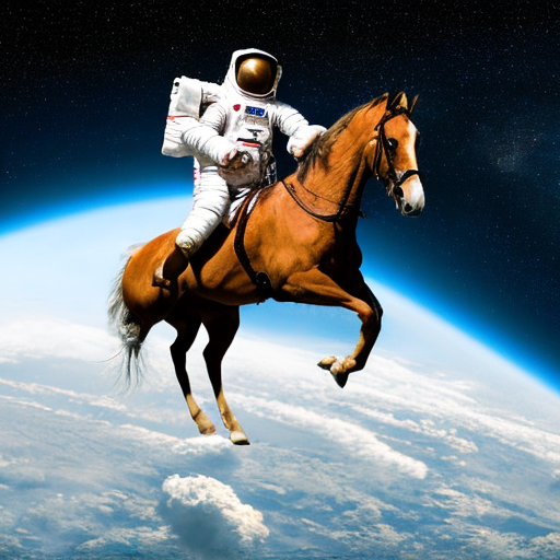

现在你就拥有了我们使用文本编码器、VAE 和 U-Net 实现的稳定扩散！

原文链接：组装自己的稳定扩散 - BimAnt