3. Classification

Given a collection of records (training set)
– each record contains a set of attributes
– one of the attributes is the class (label) that should be predicted
Find a model for class attribute as a function of the values of other attributes
Goal: previously unseen records should be assigned a class as accurately as possible
Application area: Direct Marketing, Fraud Detection
Why need it?
Classic programming is not so easy due to missing knowledge and difficult formalization as an algorithm

3.1 Definition

Given: a set of labeled records, consisting of
• data fields (a.k.a. attributes or features)
• a class label (e.g., true/false)
Generate: a function which can be used for classifying previously unseen records
• input: a record
• output: a class label

3.2 k Nearest Neighbors

The k nearest neighbors of a record x are data points that have the k smallest distance to x.
require: stored records, distance metric, value of k
steps: Compute distance to each training record -> Identify k nearest neighbors –> Use class labels of nearest neighbors to determine the class label of unknown record by taking majority vote or weighing the vote according to distance

choose k
Rule of thumb: Test k values between 1 and 10.
k too small -> sensitive to noise point
k too large -> neighborhood may include points from other classes

It’s very accurate but slow as training data needs to be searched. Can handle decision boundaries that are not parallel to the axes.

3.3 Nearest Centroids = Rocchio classifier

assign each data point to nearest centroid (center of all points of that class) 每个类别视为一个点（质心），然后在测试阶段，根据未标记数据点与这些质心的距离来决定数据点所属的类别。Nearest Centroid is a simple classification algorithm that calculates the centroid (average position) of each class based on training data. During testing, it classifies new instances by assigning them to the class whose centroid is closest.

k-NN vs. Nearest Centroid
k-NN

• slow at classification time (linear in number of data points)
• requires much memory (storing all data points)
• robust to outliers

Nearest Centroid

• fast at classification time (linear in number of classes)
• requires only little memory (storing only the centroids)
• robust to label noise
• robust to class imbalance

Which classifier is better? Strongly depends on the problem at hand!

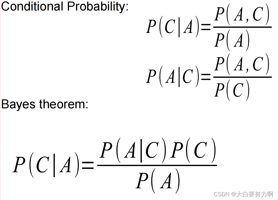
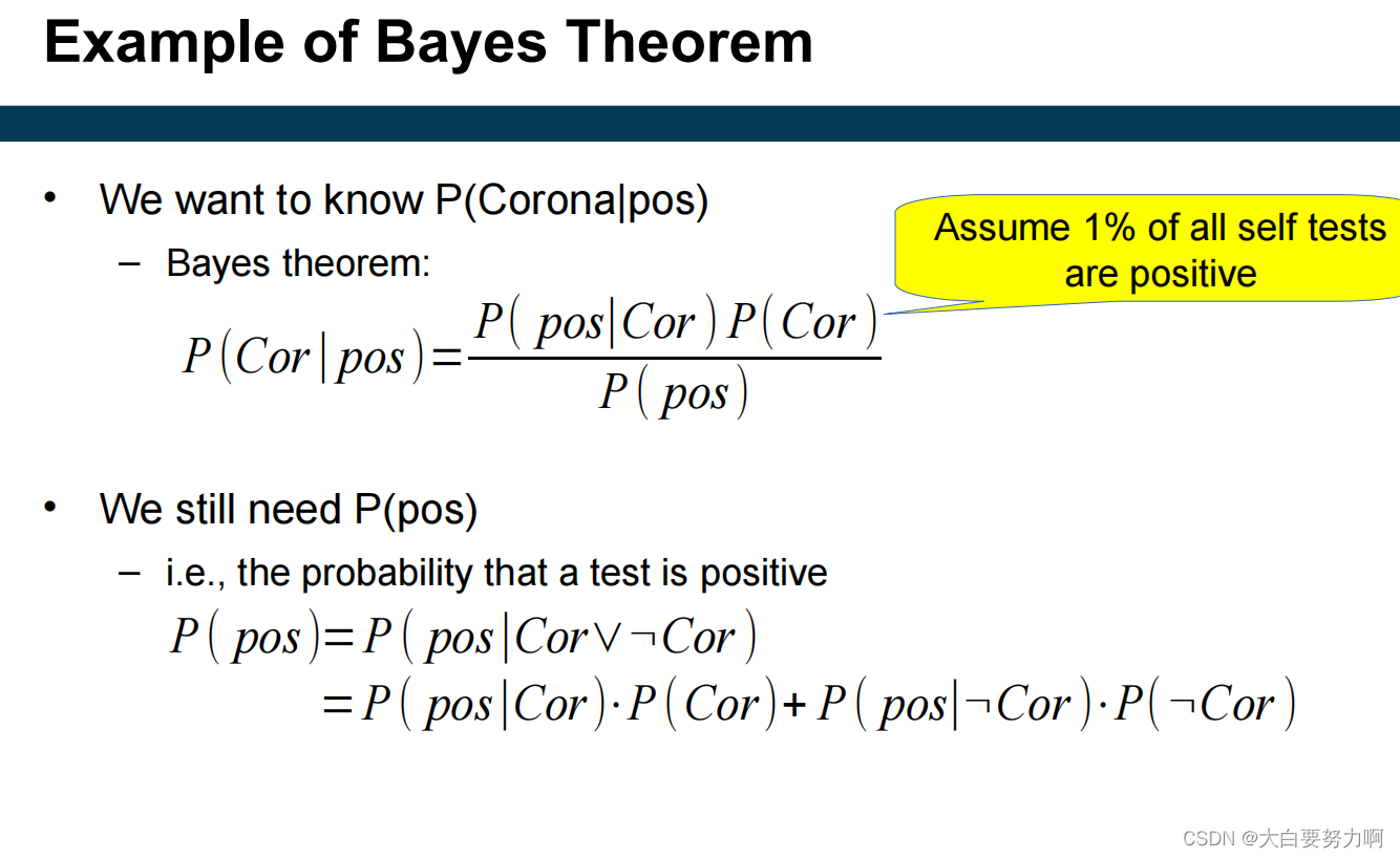
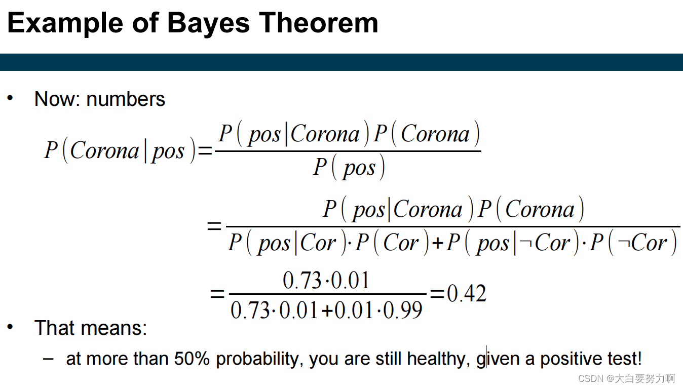
3.4 Bayes Classifier

P(C|A): conditional probability (How likely is C, given that we observe A)

Estimating the Prior Probability P(C )
counting the records in the training set that are labeled with class Cj, dividing the count by the overall number of records
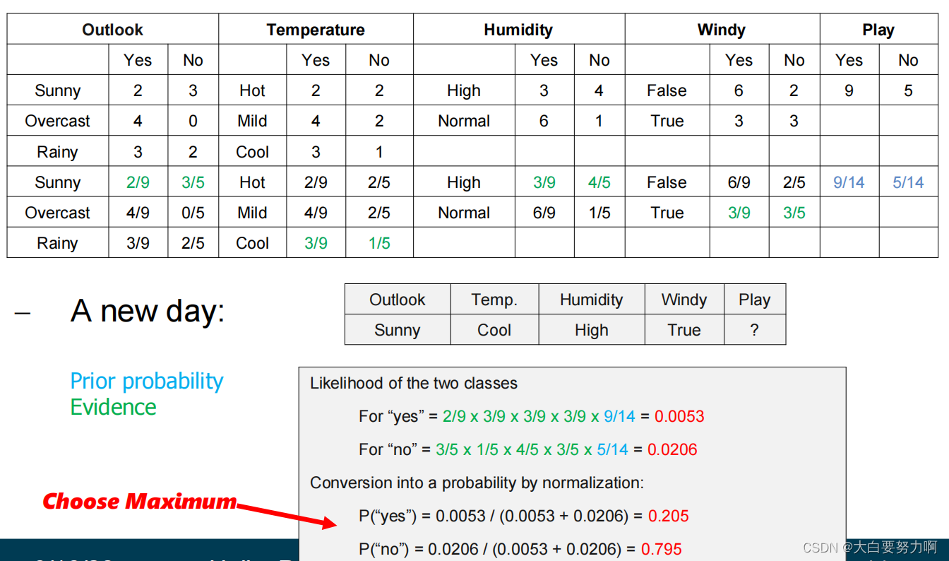
Estimating the Conditional Probability P(A | C)
Naïve Bayes assumes that all attributes are statistically independent
The independence assumption allows the joint probability P(A|C) to be reformulated as the product of the individual probabilities P(Ai|Cj).
P(A1,A2,…A3|Cj) = P(A1|Cj) * P(A2|Cj) * … * P(An|Cj)
Estimating the Probabilities P(Ai|Cj)
count how often an attribute value co-occurs with class Cj, divide by the overall number of instances in class Cj

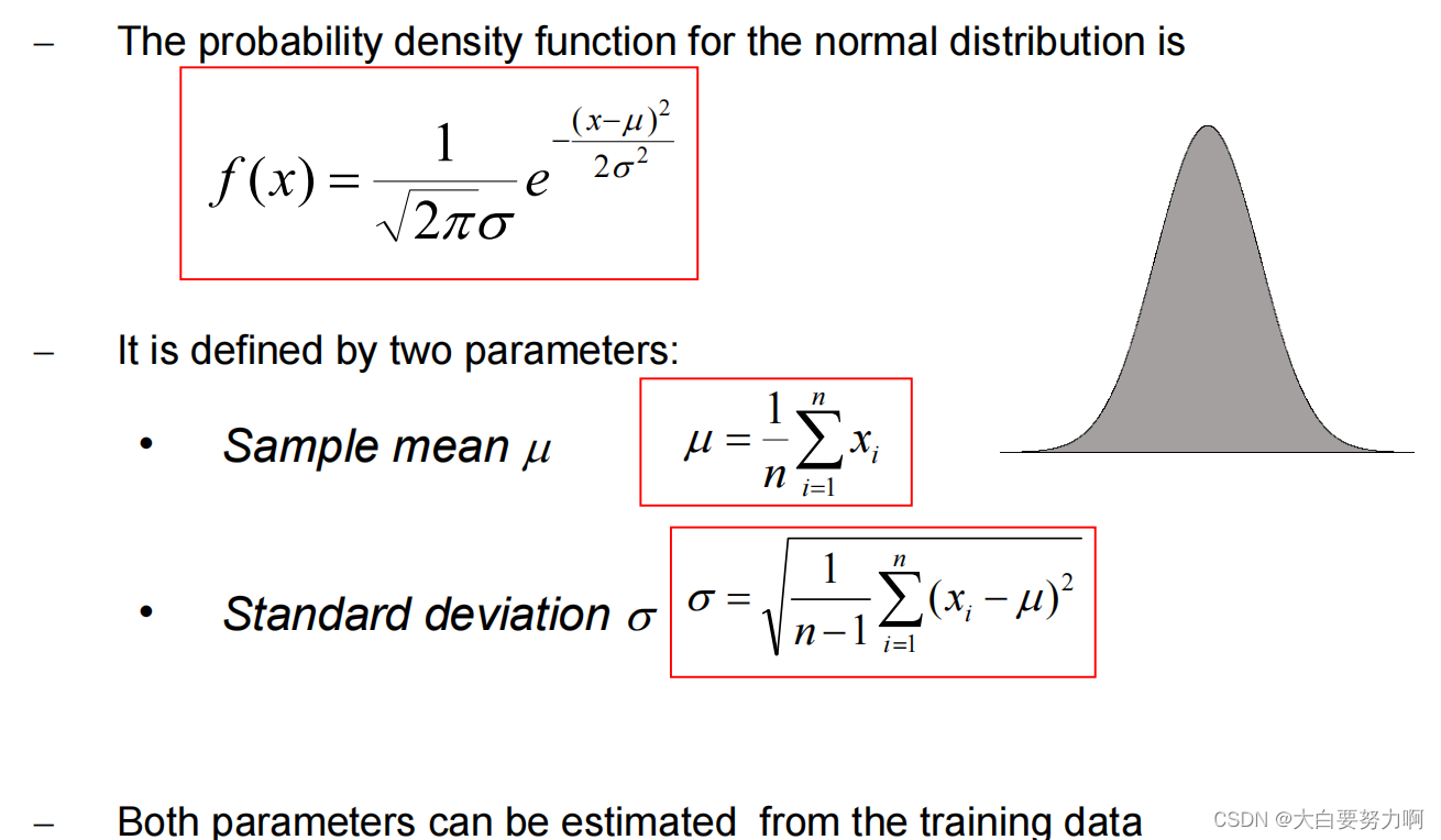
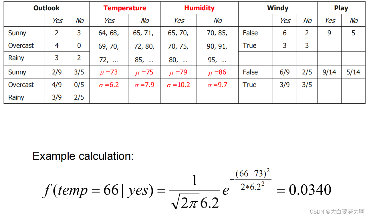
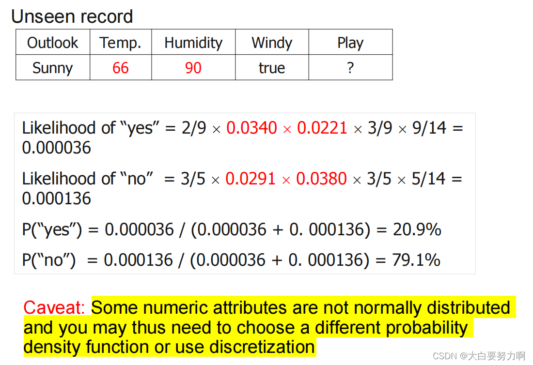
Handling Numerical Attributes
1.Discretize numerical attributes before learning classifier.
2.Make assumption that numerical attributes have a normal distribution given the class.
Use training data to estimate parameters of the distribution (e.g., mean and standard deviation)
Once the probability distribution is known, it can be used to estimate the conditional probability P(Ai|Cj)

Handling Missing Values
Missing values may occur in training and in unseen classification records. 一定要对缺失值进行处理

Zero Frequency Problem
one of the conditional probabilities is zero -> the entire expression becomes zero
It is not unlikely that an exactly same data point has not yet been observed. 有可能存在尚未观察到完全相同的数据点，因此概率有可能是0。
解决方法：Laplace Smoothing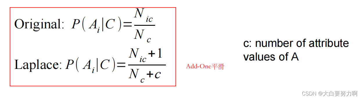

Decision Boundary of Naive Bayes Classifier

Summary

• Robust to isolated noise points
• Handle missing values by ignoring the instance during probability estimate calculations在概率估计计算过程中，通过忽略具有缺失值的实例来处理缺失值
• Robust to irrelevant attributes [reasons: the probabilistic framework + conditional independence assumption + probability smoothing techniques]
• Independence assumption may not hold for some attributes [Use other techniques such as Bayesian Belief Networks (BBN)]

Naïve Bayes works surprisingly well even if independence assumption is clearly violated [Reasons: Robustness to Violations + Effective Classification + Maximum Probability Assignment + Simple and Efficient]

Too many redundant attributes will cause problems. Solution: Select attribute subset as Naïve Bayes often works as well or better with just a fraction of all attributes.

Technical advantages:
(1) Learning Naïve Bayes classifiers is computationally cheap (probabilities are estimated in one pass over the training data)
(2) Storing the probabilities does not require a lot of memory

Redundant Variables
Violate independence assumption in Naive Bayes [Can, at large scale, skew the result]
May also skew the distance measures in k-NN, but the effect is not as drastic (Depends on the distance measure used)

Irrelevant Variables
For Naive Bayes: p(x=v|A) = p(x=v|B) for any value v, since it is random, it does not depend on the class variable. The overall result does not change

kNN vs. Naïve Bayes

	kNN	Naïve Bayes
computation	\	faster
data	less sensitive to outliers	use all data, less sensitive to label noise
redundant attributes	less problematic	\
irrelevant attributes	\	less problematic
pre-selection	yes	yes

3.5 Lazy vs. Eager Learning

K-NN is a “lazy” methods.
They do not build an explicit model! “learning” is only performed on demand for unseen records.
Nearest Centroid and Naive Bayes are simple “eager” methods （also: decision tree, rule sets, …）
classify unseen instances, learn a model

3.6 Model Evaluation

3.6.1 Metrics for Performance Evaluation

Confusion Matrix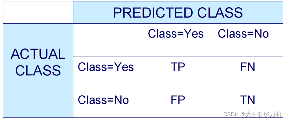

Accuracy & Error Rate

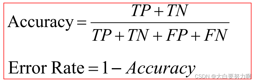
Baseline: naive guessing(always predict majority class)

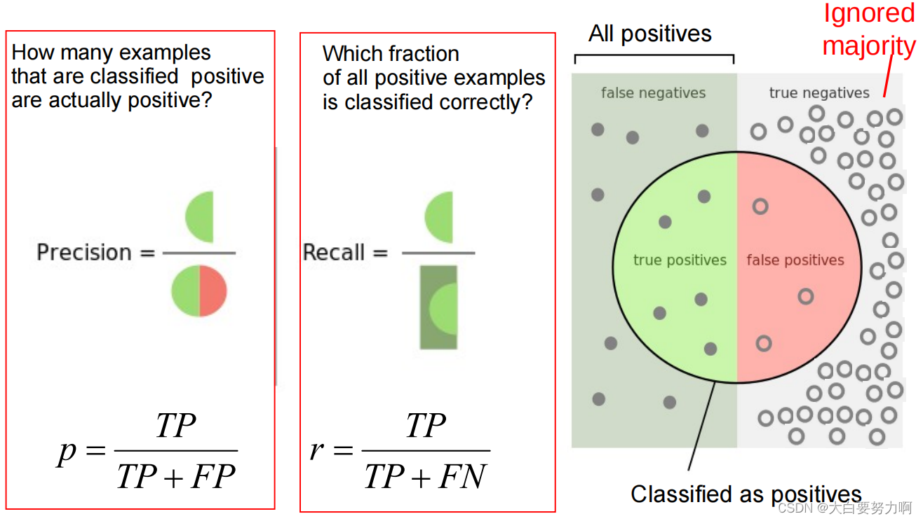
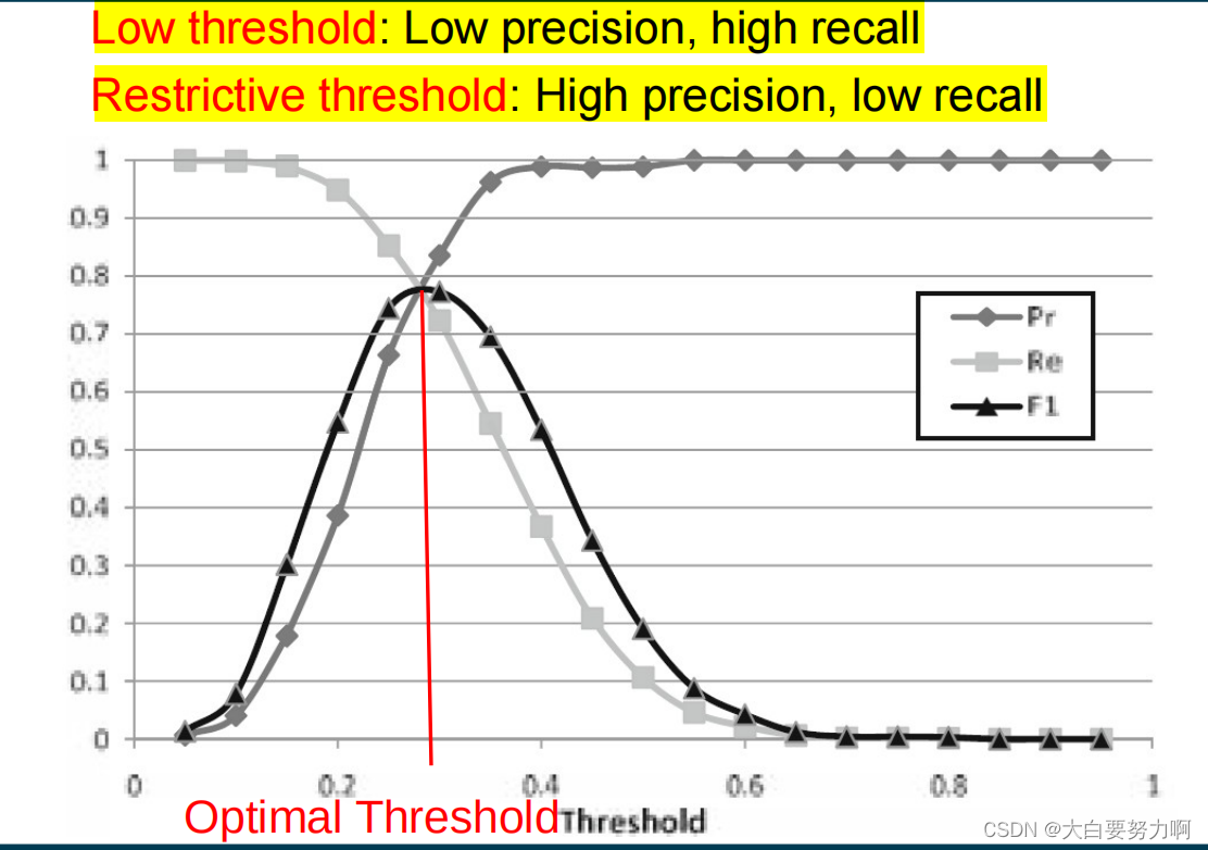
3.6.2 Limitation of Accuracy: Unbalanced Data

1. Precision & Recall

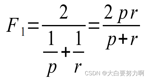
2. F1-Measure越大越好
F1-Score combines precision and recall into one measure by using harmonic mean (tends to be closer to the smaller of the two)
For F1-value to be large, both p and r must be large. 当 Precision 和 Recall 都很高时，F1 score 也会趋向于高值，表示模型在正类别和负类别的预测中取得了较好的平衡。

confidence scores: how sure the algorithms is with its prediction
3. ROC Curves:

1. Sort classifications according to confidence scores对于每个测试样本，模型输出一个置信度分数，例如，在朴素贝叶斯中可能是预测的概率。首先，将所有测试样本按照这些置信度分数从高到低排序。
2. Evaluate
   correct prediction -> draw one step up如果模型的预测是正确的，将 ROC 曲线向上移动一步（增加真正例率）。
   incorrect prediction -> draw one step to the right如果模型的预测是错误的，将 ROC 曲线向右移动一步（增加假正例率）。
   

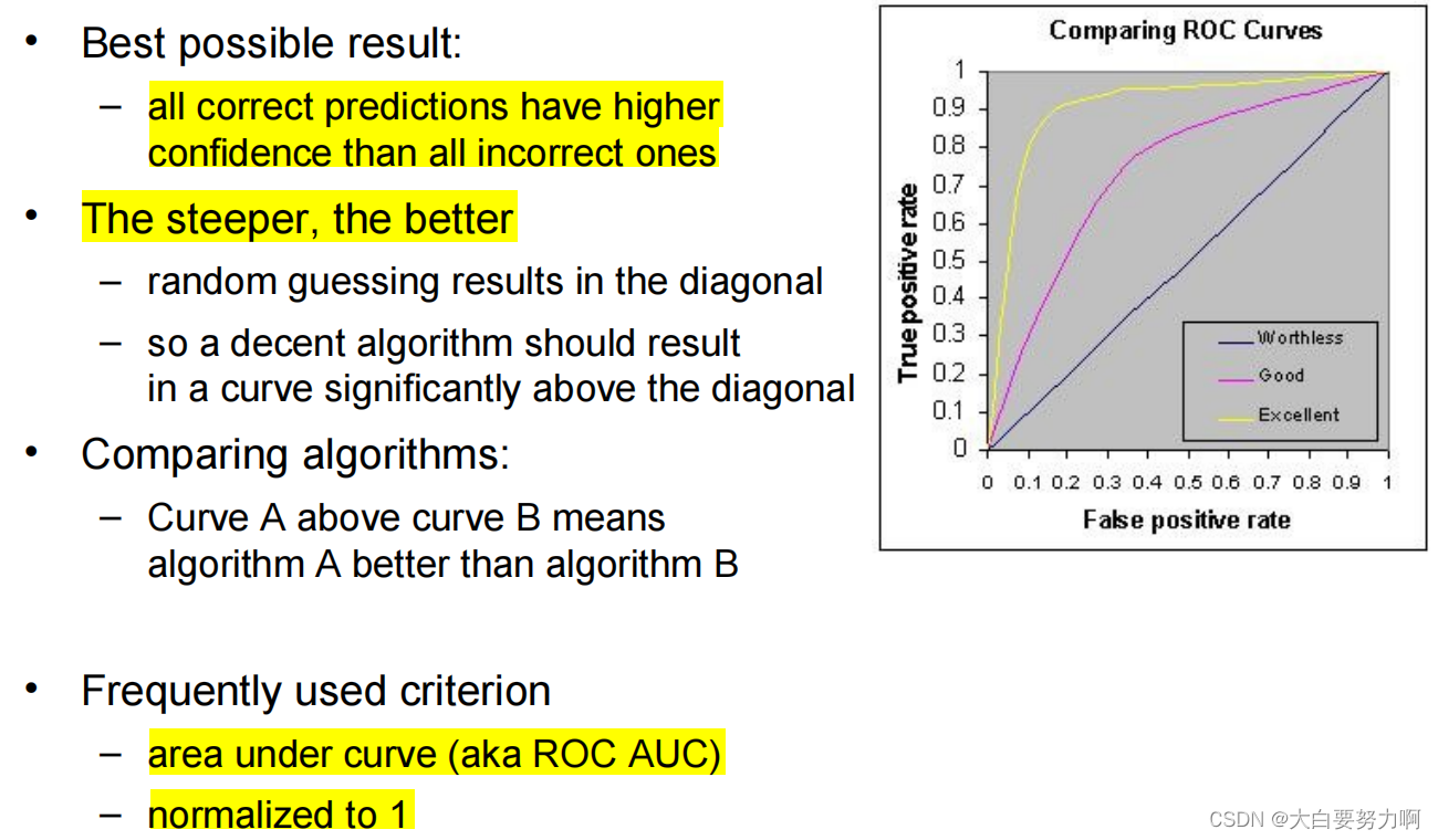
False Positive Rate是指在所有实际为负例的样本中，被错误地判定为正例的比例，FPR = FP / (FP+TN)
True Positive Rate指在所有实际为正例的样本中，被正确地判定为正例的比例=召回率，TPR = TP / (TP+FN)
曲线越接近左上角： 表示模型性能越好，具有更高的TPR和更低的FPR。
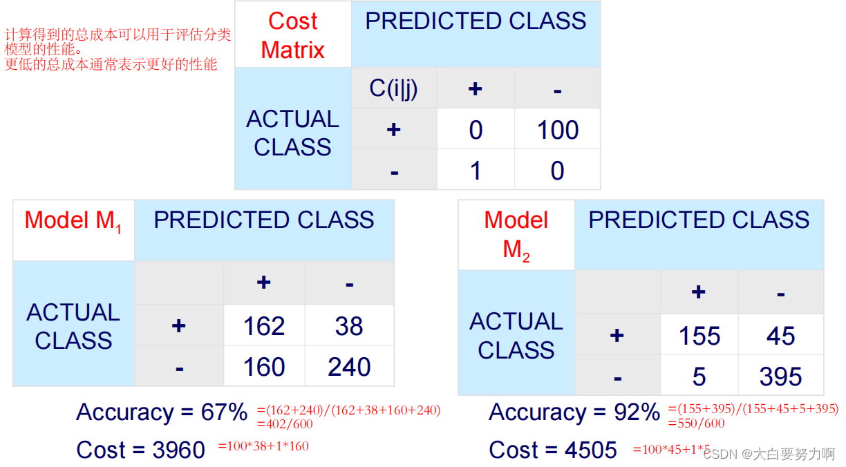
4. Cost Matrix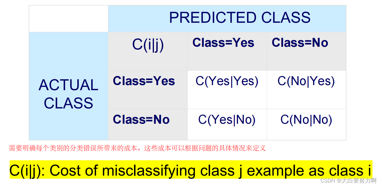

3.7 Decision Tree Classifiers

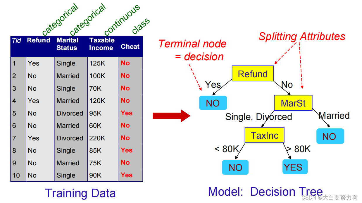
There can be more than one tree that fits the same data!
Decision Boundary
Decision boundary: border line between two neighboring regions of different classes.
Decision boundary is parallel to axes because test condition involves a single attribute at-a-time
Finding an optimal decision tree is NP-hard
Tree building algorithms use a greedy, top-down, recursive partitioning strategy to induce a reasonable solution, also known as: divide and conquer. For example, Hunt’s Algorithm, ID3, CHAID, C4.5

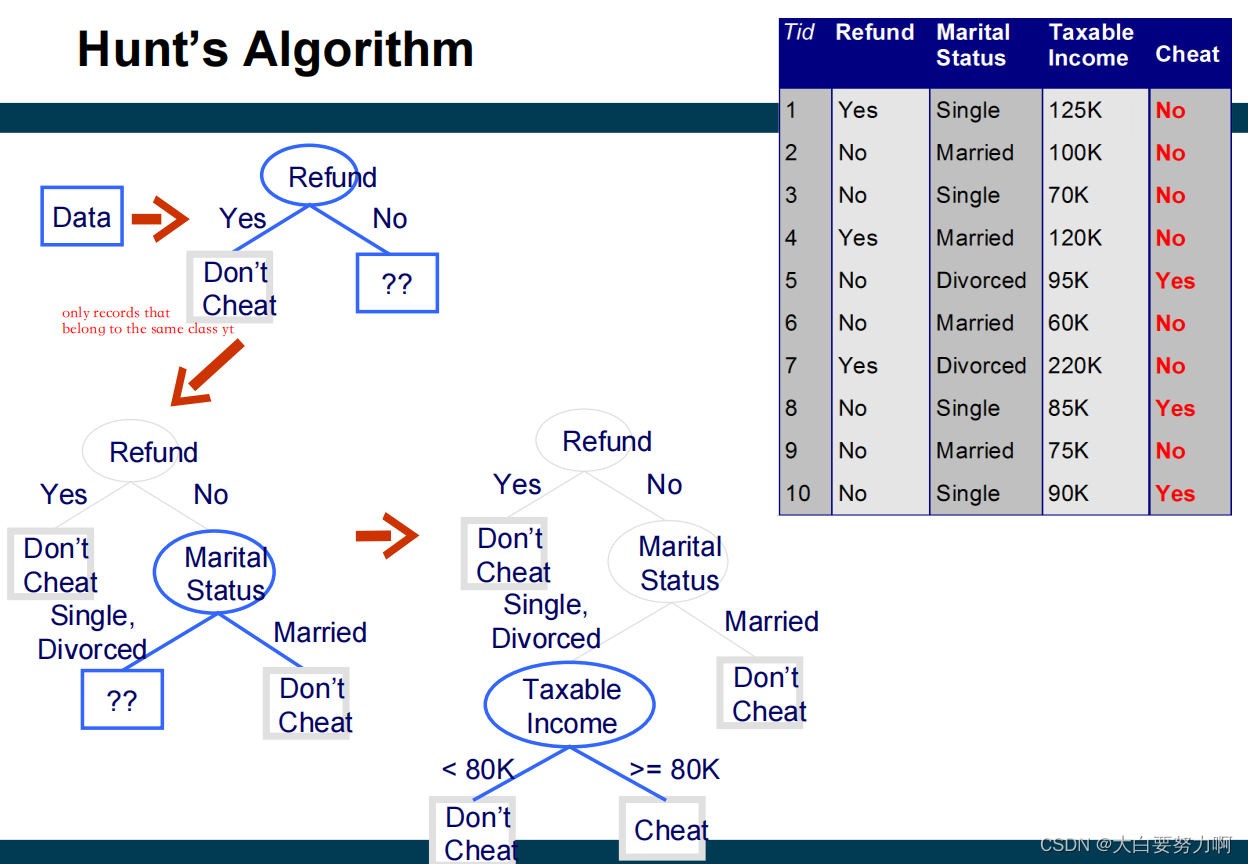
3.7.1 Hunt’s Algorithm

Let Dt be the set of training records that reach a node t.
General Procedure:
If Dt contains only records that belong to the same class yt, then t is a leaf node labeled as yt
If Dt contains records that belong to more than one class, use an attribute test to split the data into smaller subsets
Recursively apply the procedure to each subset

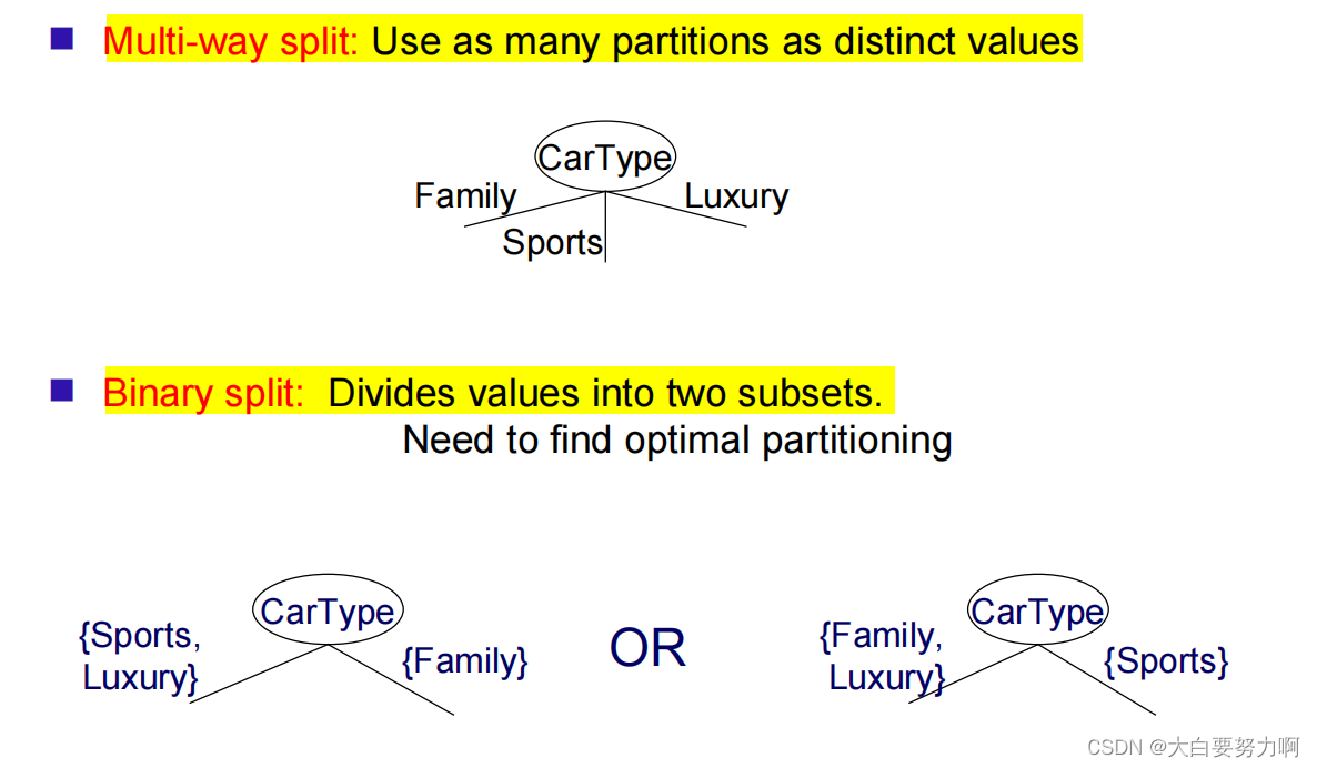
3.7.2 Split

Splitting Based on Nominal Attributes

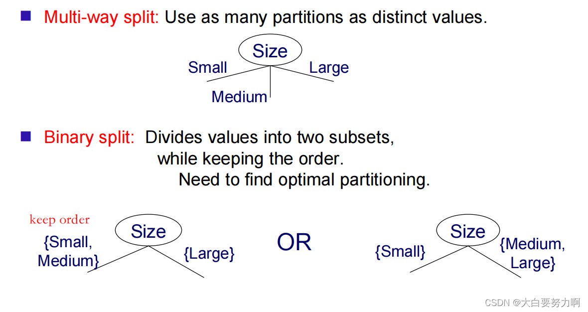
Splitting Based on Ordinal Attributes

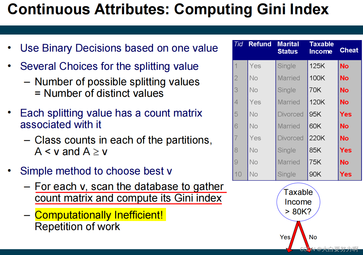
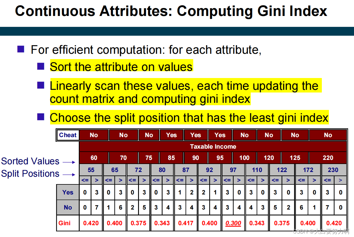
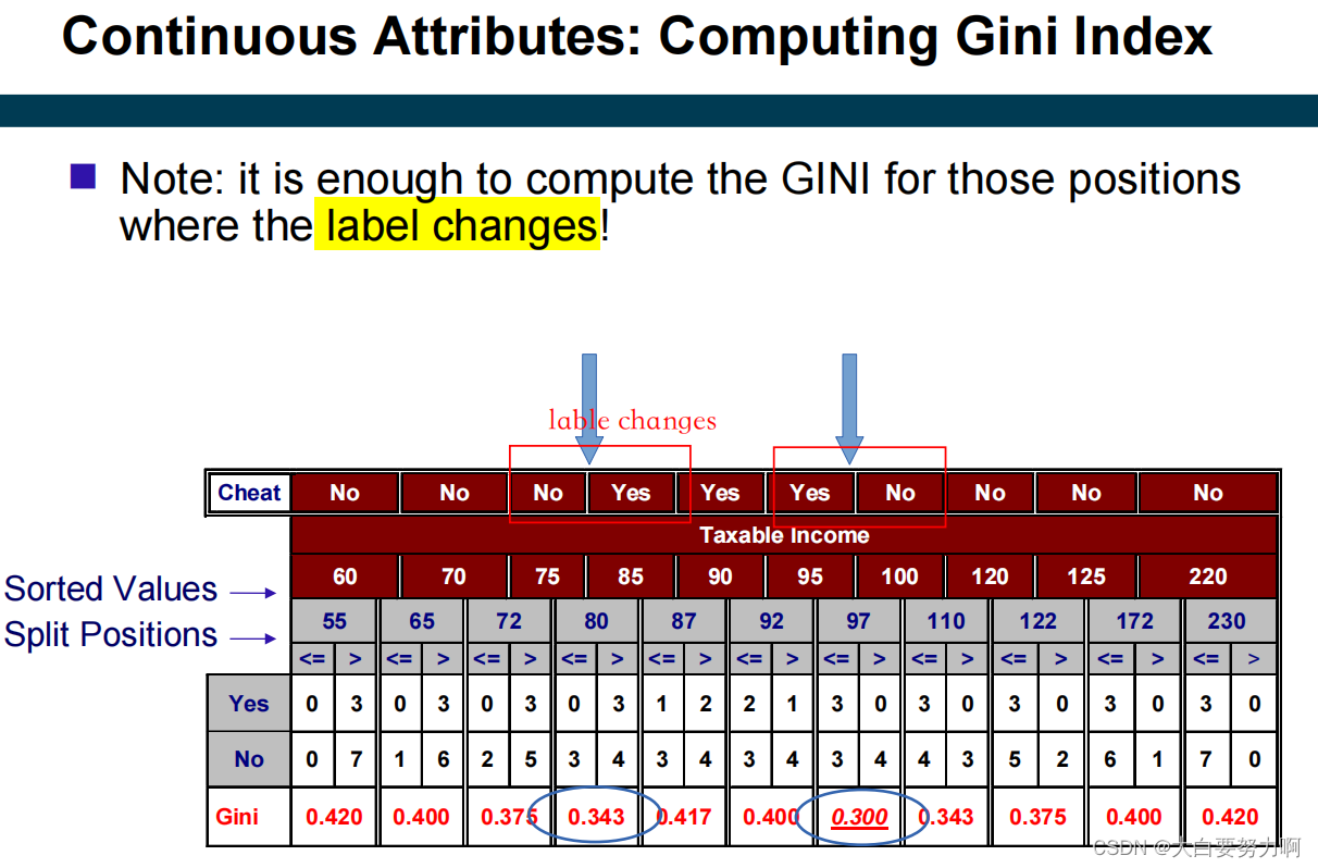
Splitting Based on Continuous Attributes

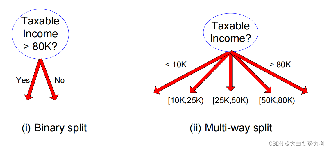
Discretization to form an ordinal categorical attribute
equal-interval binning
equal-frequency binning
binning based on user-provided boundaries

Binary Decision: (A < v) or (A > v)
usually sufficient in practice
consider all possible splits
find the best cut (i.e., the best v) based on a purity measure
can be computationally expensive

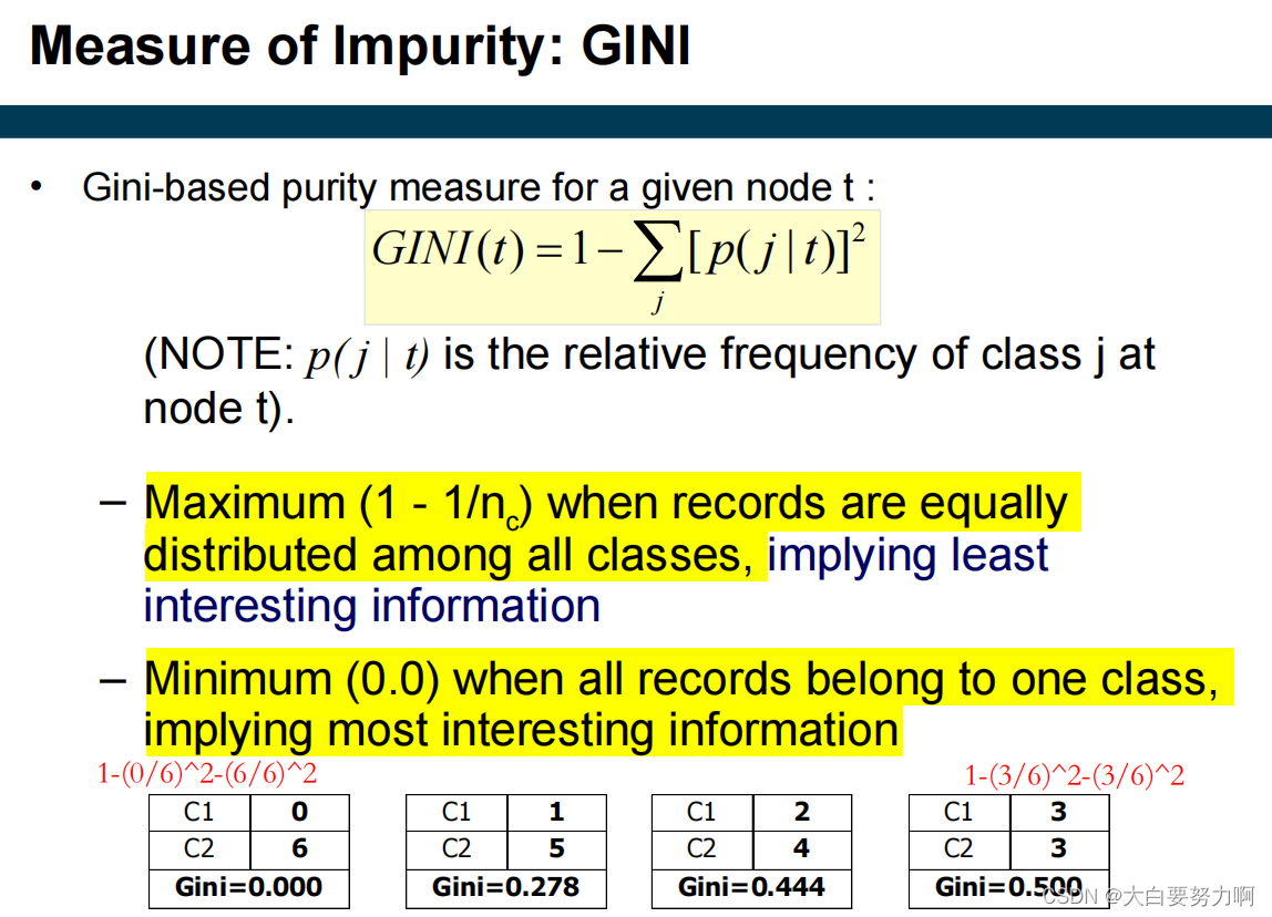
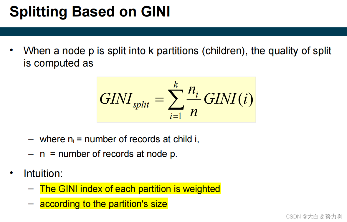
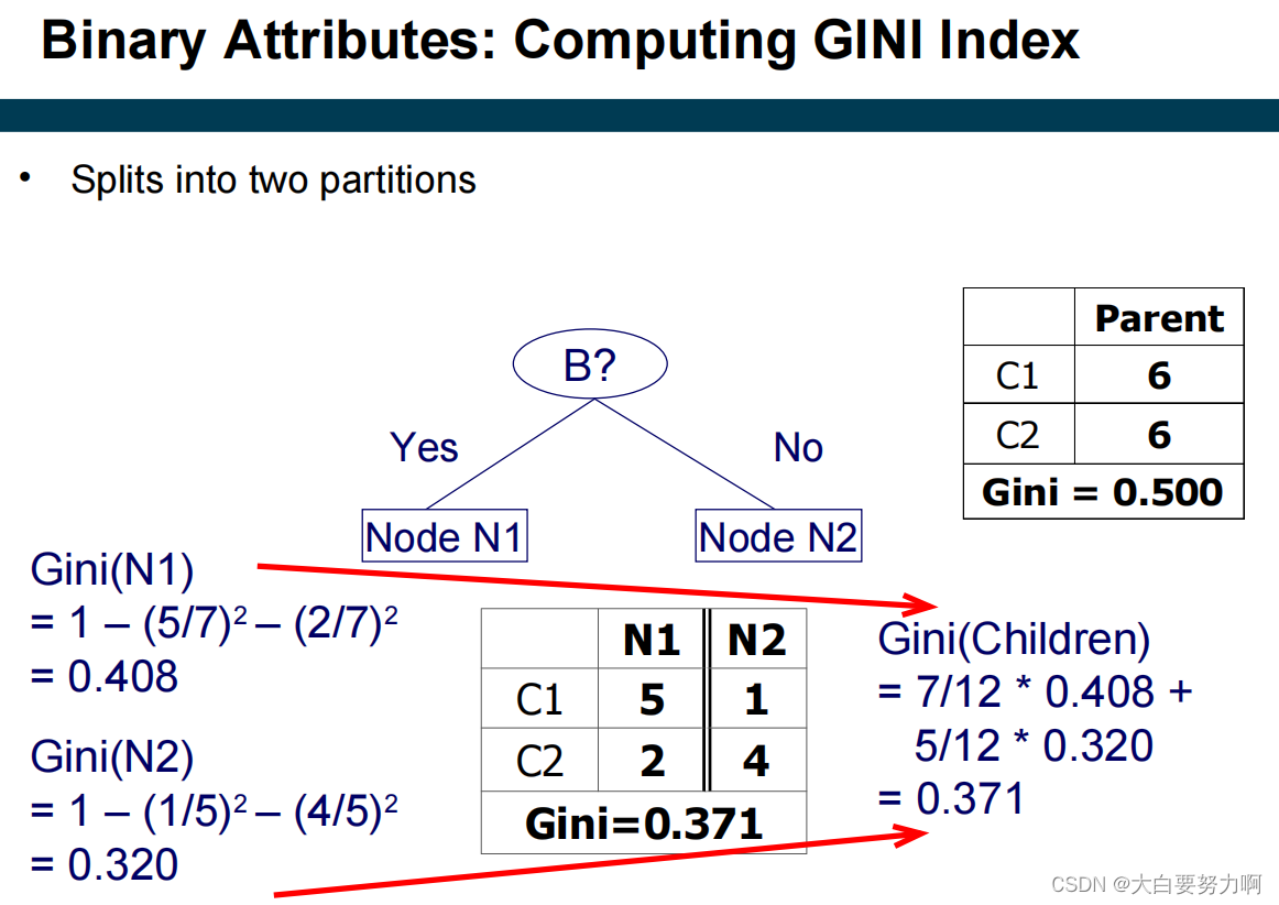
3.7.3 Common measures of node impurity

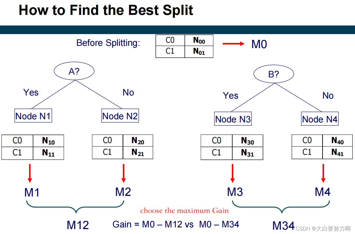
How to determine the Best Split?
Nodes with homogeneous class distribution are preferred. Need a measure of node impurity.
1. Gini Index

Binary Attributes

Continuous Attributes

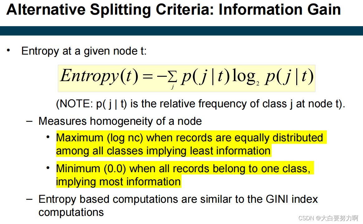
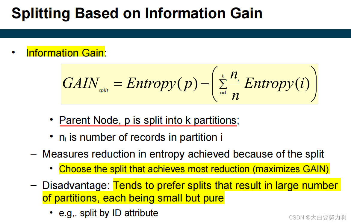
2. Entropy (Information Gain)

Decision Tree Advantages & Disadvantages
Advantages: Inexpensive to construct; Fast at classifying unknown records; Easy to interpret by humans for small-sized trees; Accuracy is comparable to other classification techniques for many simple data sets
Disadvantages: Decisions are based only one a single attribute at a time; Can only represent decision boundaries that are parallel to the axes

Decision Tree vs. k-NN

	k-NN	Decision Tree
Decision Boundaries	arbitrary	rectangular
Sensitivity to Scales	need normalization	does not need normalization
Runtime & Memory	cheap to train but expensive for classification	expensive to train but cheap for classification

3.8 Overfitting

Overfitting: Good accuracy on training data, but poor on test data.
Symptoms: Tree too deep and too many branches
Typical causes of overfitting: too little training data, noise, poor learning algorithm
Which tree do you prefer?
Occam’s Razor
If you have two theories that explain a phenomenon equally well, choose the simpler one!

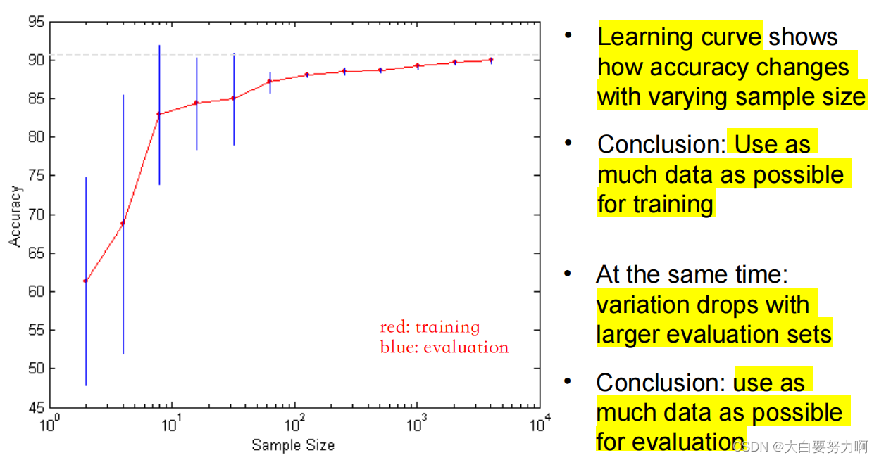
Learning Curve

Holdout Method
The holdout method reserves a certain amount for testing and uses the remainder for training
Typical: one third for testing, the rest for training

For unbalanced datasets (few or none instances of some classes), samples might not be representative. -> Stratified sample: balances the data - Make sure that each class is represented with approximately equal proportions in both subsets. Other attributes may also be considered for stratification, e.g., gender, age, …

Leave One Out
Iterate over all examples
– train a model on all examples but the current one
– evaluate on the current one
每个样本都被当作测试集，而其余的样本组成训练集。这个过程会重复执行，直到每个样本都被作为测试集被验证过一次。
Yields a very accurate estimate but is computationally infeasible in most cases

Cross-Validation (k-fold cross-validation)
Compromise of Leave One Out and decent runtime
Cross-validation avoids overlapping test sets
Steps:
Step 1: Data is split into k subsets of equal size (Stratification may be applied)
Step 2: Each subset in turn is used for testing
and the remainder for training
The error estimates are averaged to yield an overall error estimate
Frequently used value for k : 10 (the gold standard for folds was long set to 10)

How to Address Overfitting?

1. Pre-Pruning (Early Stopping Rule)
   Stop the algorithm before it becomes a fully-grown tree
   Typical stopping conditions for a node: Stop if all instances belong to the same class or Stop if all the attribute values are the same
   Less restrictive conditions: Stop if number of instances within a node is less than some user-specified threshold or Stop if expanding the current node only slightly improves the impurity measure (user-specified threshold)
2. Post-pruning
   Grow decision tree to its entire size -> Trim the nodes of the decision tree in a bottom-up fashion [ using a validation data set or an estimate of the generalization error ] -> If generalization error improves after trimming [ replace sub-tree by a leaf node / Class label of leaf node is determined from majority class of instances in the sub-tree]

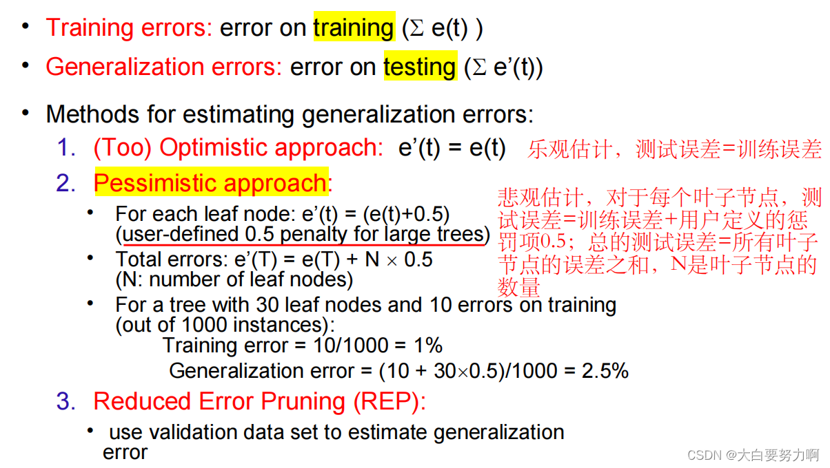
Training vs. Generalization Errors
Training error = resubstitution error = apparent error: errors made in training, misclassified training instances -> can be computed
Generalization error: errors made on unseen data, no apparent evidence -> must be estimated

Estimating the Generalization Error

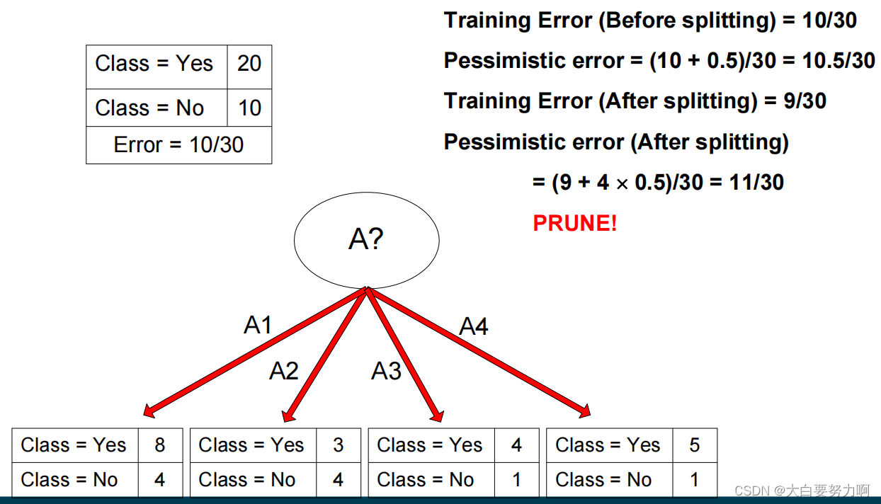
Example of Post-Pruning

3.9 Alternative Classification Methods

Some cases are not nicely expressible in trees and rule sets.(Example: if at least two of Employed, Owns House, and Balance Account are yes → Get Credit is yes)

3.9.1 Artificial Neural Networks (ANN)

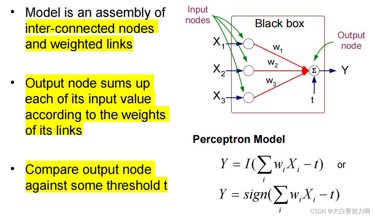
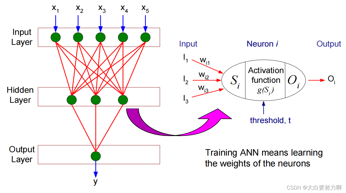
Decision Boundaries of ANN: Arbitrarily shaped objects & Fuzzy boundaries

3.9.2 Support Vector Machines

Find a linear hyperplane (decision boundary) that will separate the data.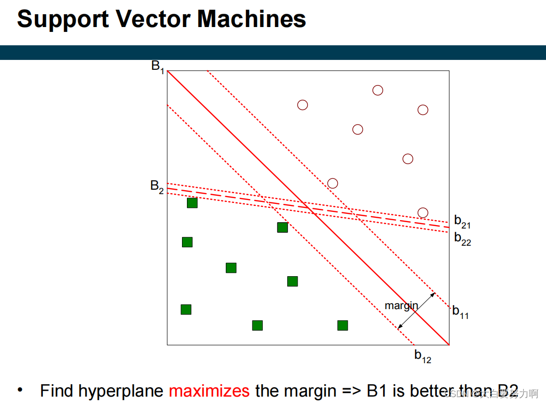

What is computed?
a separating hyper plane, defined by its support vectors (hence the name)

“support vectors” refer to the training data points that are crucial in defining the decision boundary (or hyperplane).
Challenges: Computing an optimal separation is expensive and it requires good approximations
Dealing with noisy data: introducing “slack variables” in margin computation

3.9.3 Nonlinear Support Vector Machines

• Transform data into higher dimensional space将输入数据从原始特征空间映射到更高维的空间
• Transformation in higher dimensional space
  Kernel function
  Different variants: polynomial function, radial basis function, …
• Finding a hyperplane in higher dimensional space

3.10 Hyperparameter Selection

A hyperparameter is a parameter which influences the learning process and whose value is set before the learning begins. For example, pruning thresholds for trees and rules; gamma and C for SVMs; learning rate, hidden layers for ANNs.
parameters are learned from the training data. For example, weights in an ANN, probabilities in Naïve Bayes, splits in a tree.

How to determine good hyperparameters?
(1) manually play around with different hyperparameter settings
(2) have your machine automatically test many different settings(Hyperparameter Optimization)

Hyperparameter Optimization
Goal: Find the combination of hyperparameter values that results in learning the model with the lowest generalization error
How to determine the parameter value combinations to be tested?

• Grid Search: Test all combinations in user-defined ranges
• Random Search: Test combinations of random parameter values
• Evolutionary Search: Keep specific parameter values that worked well

3.11 Model Selection

From all learned models M, select the model mbest that is expected to generalize best to unseen records

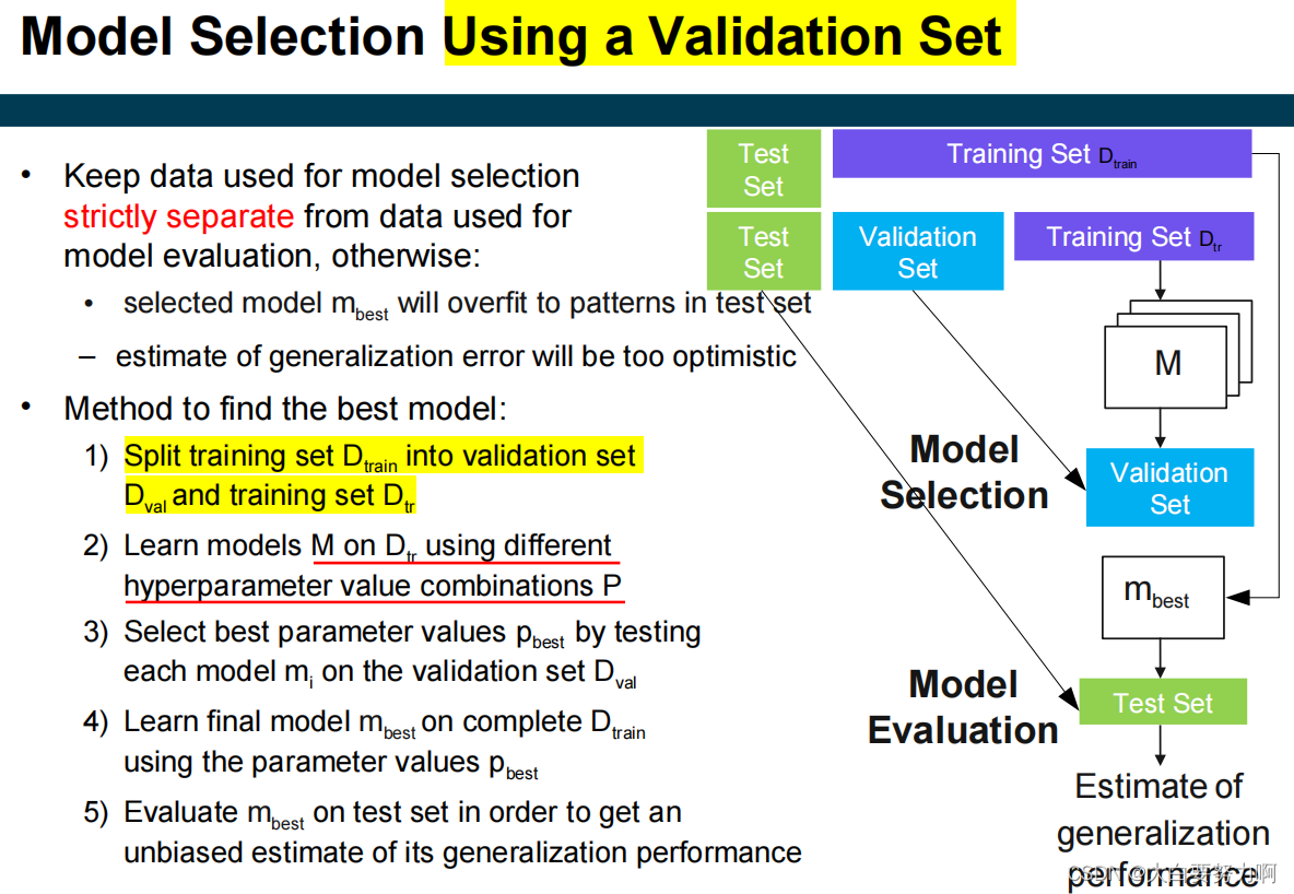
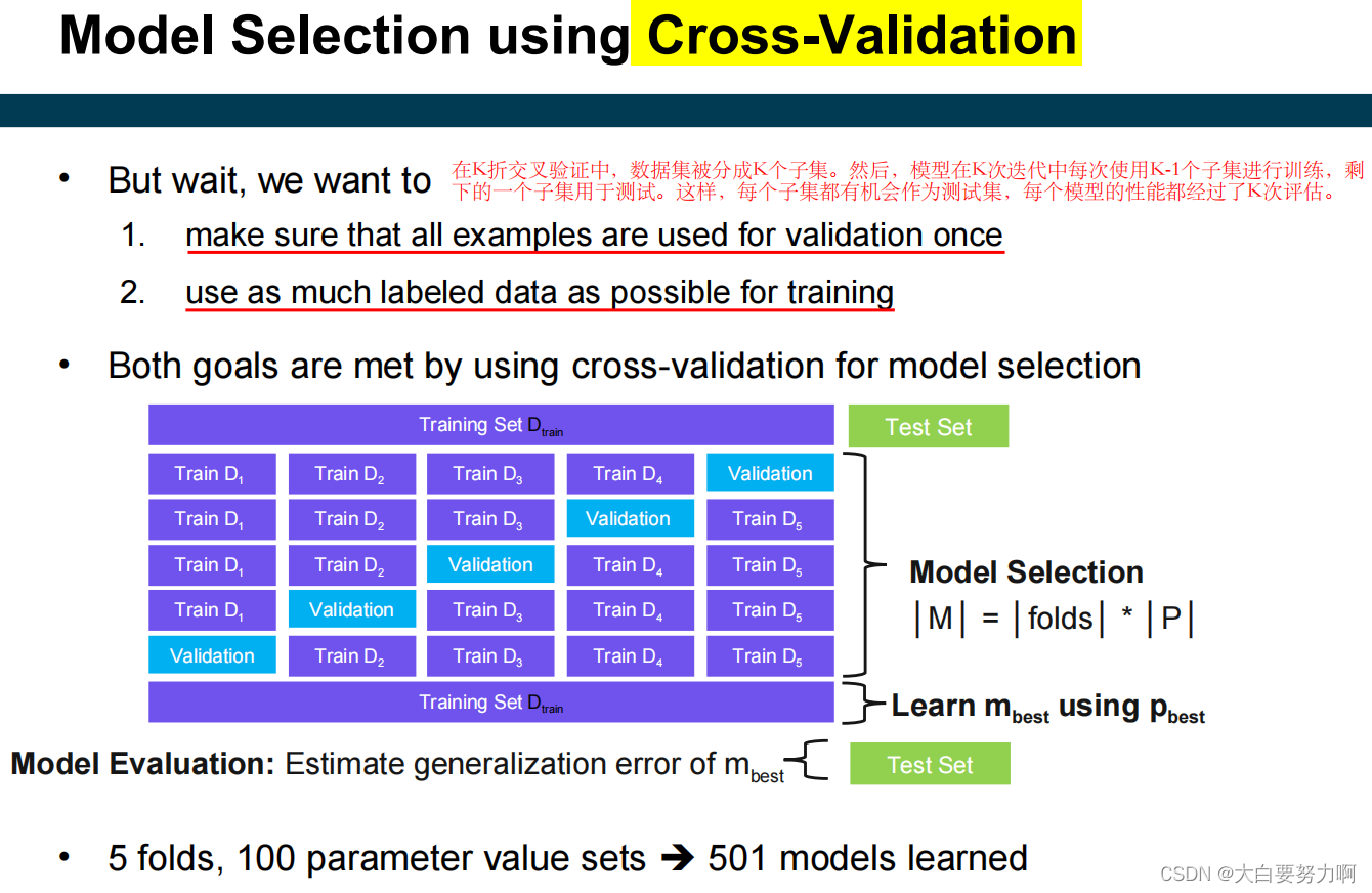
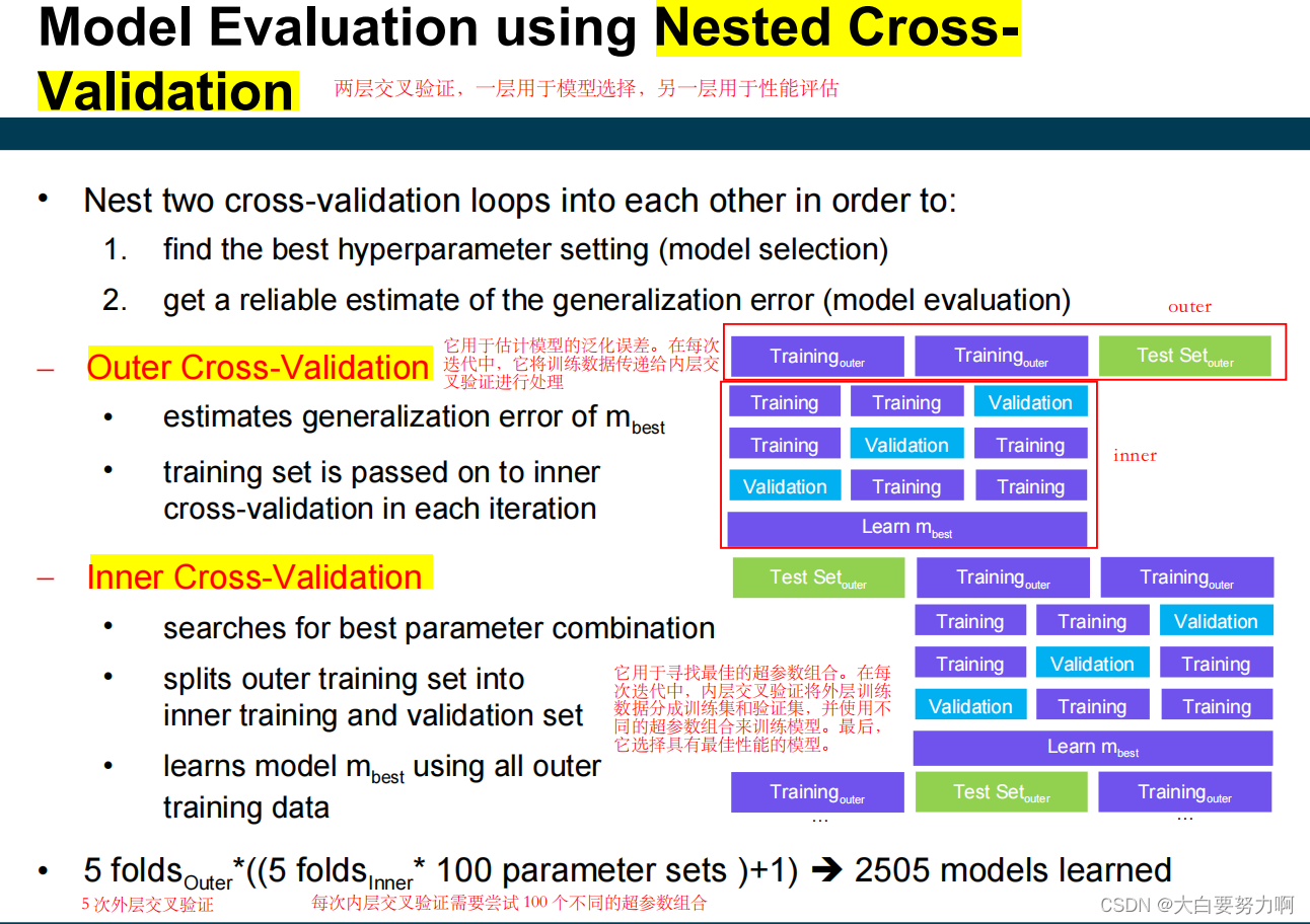
grid search for model selection
cross-validation for model evaluation