1. 入门案例：LinearPolicyGraph

看一个简单的数值优化的例子：

我们将其建立为一个N阶段的问题：

初始值为M。
使用SDDP.jl进行求解：

using SDDP
import IpoptM, N = 5, 3model = SDDP.LinearPolicyGraph(stages = N,lower_bound = 0.0,optimizer = Ipopt.Optimizer,
) do subproblem, node@variable(subproblem, s >= 0, SDDP.State, initial_value = M)@variable(subproblem, x >= 0)@stageobjective(subproblem, x^2)@constraint(subproblem, x <= s.in)@constraint(subproblem, s.out == s.in - x)if node == Nfix(s.out, 0.0; force = true)endreturn
endSDDP.train(model)
println(SDDP.calculate_bound(model))
simulations = SDDP.simulate(model, 1, [:x])
for data in simulations[1]println("x_$(data[:node_index]) = $(data[:x])")
end

结果为

8.333333297473812
x_1 = 1.6666655984419778
x_2 = 1.6666670256548375
x_3 = 1.6666673693365108

非常接近理论最优值。

2 报童模型：加入随机变量

报童每天早上进一批报纸，需求有个大致的数，但是并不确定。那么报童要进多少报纸合适？
变量如下：

• 报纸成本c，零售价v
• 残值s，缺货损失p
• 需求为随机变量x，概率密度为f
• 决策变量为订货量Q
• 目标函数为max(利润-成本)，假如x>Q，则利润=vQ，成本=cQ+p(x-Q)
• 最佳订货量Q满足到Q的概率积分=(v+p-c)/(v+p-s)，推倒过程这里忽略

.我们缺货无损失，残值为0，零售价30.5，订货价20.5，则最佳订货量满足积分=0.328。若f为均值300，方差50的正态分布函数，则最佳订货量 = -0.445*50+300 = 278
我们使用Julia进行求解，首先要将正态分布离散化：

using Distributions,StatsPlots
D = Distributions.Normal(300,50)
N = 1000
d = rand(D, N)
P = fill(1 / N, N)
StatsPlots.histogram(d; bins = 80, label = "", xlabel = "Demand")

接下来是一个trick，这里是先决策再实现随机变量，因此把问题建成两阶段的模型，第一阶段决策为购买量u_make，第二阶段实现随机变量ω，随后决策为销售量u_sell。
模型如下：

using SDDP, HiGHS
model = SDDP.LinearPolicyGraph(;stages = 2,sense = :Max,upper_bound = 20 * maximum(d),  # The `M` in θ <= Moptimizer = HiGHS.Optimizer,
) do subproblem::JuMP.Model, stage::Int@variable(subproblem, x >= 0, SDDP.State, initial_value = 0)if stage == 1@variable(subproblem, u_make >= 0, Int)@constraint(subproblem, x.out == x.in + u_make)@stageobjective(subproblem, -20.5 * u_make)else@variable(subproblem, u_sell >= 0, Int)@constraint(subproblem, u_sell <= x.in)@constraint(subproblem, x.out == x.in - u_sell)# 把连续随机变量离散化SDDP.parameterize(subproblem, d, P) do ωset_upper_bound(u_sell, ω)returnend@stageobjective(subproblem, 30.5 * u_sell)end
end
SDDP.train(model;)
rule = SDDP.DecisionRule(model; node = 1)
SDDP.evaluate(rule; incoming_state = Dict(:x => 0.0),controls_to_record = [:u_make])

输出为：
(stage_objective = -5699.0, outgoing_state = Dict(:x => 278.0), controls = Dict(:u_make => 278.0))
接下来进行仿真观察：

simulations = SDDP.simulate(model,10,  #= number of replications =#[:x, :u_make, :u_sell];  #= variables to record =#skip_undefined_variables = true,
);
simulations[1][1]

收益如下：

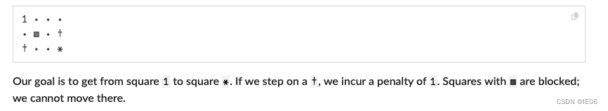
3 探索迷宫：UnicyclicGraph

首先构造一个迷宫：

M, N = 3, 4
initial_square = (1, 1)
reward, illegal_squares, penalties = (3, 4), [(2, 2)], [(3, 1), (2, 4)]
path = fill("⋅", M, N)
path[initial_square...] = "1"
for (k, v) in (illegal_squares => "▩", penalties => "†", [reward] => "*")for (i, j) in kpath[i, j] = vend
end
print(join([join(path[i, :], ' ') for i in 1:size(path, 1)], '\n'))

定义P为所有满足可以移动到 (i, j)的(a, b) 集合。
使用SDDP.UnicyclicGraph，定义一个无限的循环图

discount_factor = 0.9
graph = SDDP.UnicyclicGraph(discount_factor)

定义了一个不断自循环的图：

Root0
Nodes1
Arcs0 => 1 w.p. 1.01 => 1 w.p. 0.9

import HiGHSmodel = SDDP.PolicyGraph(graph;sense = :Max,upper_bound = 1 / (1 - discount_factor),optimizer = HiGHS.Optimizer,
) do sp, _# Our state is a binary variable for each square@variable(sp,x[i = 1:M, j = 1:N],Bin,SDDP.State, # 每一阶段都是M*N的状态变量initial_value = (i, j) == initial_square, # 初始位置(1,1))# 只能在一个位置@constraint(sp, sum(x[i, j].out for i in 1:M, j in 1:N) == 1)# Incur rewards and penalties# 这里reward是终点位置，penalties是所有惩罚点的位置@stageobjective(sp, x[reward...].out - sum(x[i, j].out for (i, j) in penalties))# Constraints on valid movesfor i in 1:M, j in 1:N# 允许移动的位置moves = [(i - 1, j), (i + 1, j), (i, j), (i, j + 1), (i, j - 1)]filter!(v -> 1 <= v[1] <= M && 1 <= v[2] <= N && !(v in illegal_squares), moves)# 移动出去的值不能大于其他位置进去的值的和。由于都是Bin变量，因此等价于说从i，j移动到了某个允许的a，b上@constraint(sp, x[i, j].out <= sum(x[a, b].in for (a, b) in moves))endreturn
end
SDDP.train(model)
simulations = SDDP.simulate(model,1,[:x];sampling_scheme = SDDP.InSampleMonteCarlo(max_depth = 10,#terminate_on_dummy_leaf = false,),
);
for (t, data) in enumerate(simulations[1]), i in 1:M, j in 1:Nif data[:x][i, j].in > 0.5path[i, j] = "$t"end
endprint(join([join(path[i, :], ' ') for i in 1:size(path, 1)], '\n'))

注意Simulating a cyclic policy graph requires an explicit sampling_scheme that does not terminate early based on the cycle probability。结果为：

1 2 3 ⋅
⋅ ▩ 4 †
† ⋅ 5 *

4 牛奶制造：MarkovianGraph

使用MarkovianGraph可以接受一个仿真器graph = SDDP.MarkovianGraph(simulator; budget = 30, scenarios = 10_000);
buget是node的个数，scenarios是计算转移概率时的采样个数。这里使用Markovian过程来模拟一个随时间变化的过程，node的个数需要大于stage的个数，node越多，模拟越精确。

这里问题描述如下：

• 产奶量不确定，牛奶市场价格不确定
• 需求无限。未售出的牛奶可以制成奶粉
• 公司也可以接订单，按照当前价格收款，但是4个月之后交付。届时产能不够的话，需要额外购买牛奶。
• 决策为需要接多少订单

首先我们用预测模型给出牛奶的价格，假设模型如下：

function simulator()residuals = [0.0987, 0.199, 0.303, 0.412, 0.530, 0.661, 0.814, 1.010, 1.290]residuals = 0.1 * vcat(-residuals, 0.0, residuals)scenario = zeros(12)y, μ, α = 4.5, 6.0, 0.05for t in 1:12y = exp((1 - α) * log(y) + α * log(μ) + rand(residuals))scenario[t] = clamp(y, 3.0, 9.0)endreturn scenario
endplot = Plots.plot([simulator() for _ in 1:500];color = "gray",opacity = 0.2,legend = false,xlabel = "Month",ylabel = "Price [\$/kg]",xlims = (1, 12),ylims = (3, 9),
)

用30个点模拟出来的转移概率图如下：

for ((t, price), edges) in graph.nodesfor ((t′, price′), probability) in edgesPlots.plot!(plot,[t, t′],[price, price′];color = "red",width = 3 * probability,)end
endplot

接下来给定具体数值：

• 产奶量不确定，为0.1-0.2之间的均匀分布。生产没有成本。
• 牛奶市场价格按照node进行概率转移，售出价格1倍
• 需求无限。未售出的牛奶可以制成奶粉然后在下个月以同样价格售出。
• 公司也可以接订单，按照当前价格收款，但是4个月之后交付。成本为绝对值0.01，四个月后售出价格为1.05倍
• 届时产能不够的话，需要额外购买牛奶。费用1.5倍
• 决策为需要接多少订单

建模如下：

model = SDDP.PolicyGraph(graph;# 将price用graph随机过程来模拟，不用再单独建随机变量来模拟sense = :Max,upper_bound = 1e2,optimizer = HiGHS.Optimizer,
) do sp, nodet, price = node::Tuple{Int,Float64}c_buy_premium = 1.5Ω_production = range(0.1, 0.2; length = 5)c_max_production = 12 * maximum(Ω_production)# 两个状态变量@variable(sp, 0 <= x_stock, SDDP.State, initial_value = 0) # track库存变量@variable(sp, 0 <= x_forward[1:4], SDDP.State, initial_value = 0) # track forward变化# 三个核心决策变量@variable(sp, 0 <= u_spot_sell <= c_max_production)@variable(sp, 0 <= u_spot_buy <= c_max_production);c_max_futures = t <= 8 ? c_max_production : 0.0@variable(sp, 0 <= u_forward_sell <= c_max_futures)# 一个随机变量@variable(sp, ω_production)# Forward contracting constraints:@constraint(sp, [i in 1:3], x_forward[i].out == x_forward[i+1].in)@constraint(sp, x_forward[4].out == u_forward_sell)@constraint(sp, x_stock.out == x_stock.in + ω_production + u_spot_buy - x_forward[1].in - u_spot_sell)Ω = [(price, p) for p in Ω_production]SDDP.parameterize(sp, Ω) do ω::Tuple{Float64,Float64}fix(ω_production, ω[2])@stageobjective(sp,  ω[1] * (u_spot_sell - 1.5 * u_spot_buy) +(ω[1] * 1.05 - 0.01) * u_forward_sell)returnendreturn
end

SDDP.SimulatorSamplingScheme is used in the forward pass. It generates an out-of-sample sequence of prices using simulator and traverses the closest sequence of nodes in the policy graph.翻译过来就是SimulatorSamplingScheme会根据产生的随机变量，寻找最为接近的node路径。
AVaR(β) Computes the expectation of the β fraction of worst outcomes. β must be in [0, 1]. When β=1, this is equivalent to the Expectation risk measure. When β=0, this is equivalent to the WorstCase risk measure. 翻译过来就是AVaR综合了最差情况和均值。

SDDP.train(model;time_limit = 20,risk_measure = 0.5 * SDDP.Expectation() + 0.5 * SDDP.AVaR(0.25),sampling_scheme = SDDP.SimulatorSamplingScheme(simulator),
)

我们仿真一次：

simulations = SDDP.simulate(model,200,Symbol[:x_stock, :u_forward_sell, :u_spot_sell, :u_spot_buy];sampling_scheme = SDDP.SimulatorSamplingScheme(simulator),
);
simulations[1][12]

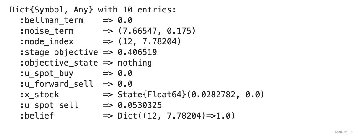
可以发现，node_index里面的price下标是7.78204， SDDP.parameterize的实际用的price是7.66547