均方差损失推导-编程知识

一、损失函数（Cost function）

定义：用于衡量模型预测结果与真实结果之间差距的函数。（有的地方称之为代价函数，但是个人感觉损失函数这个名称更贴近实际用途）

理解：（以均方差损失函数为例）

对于一个线性回归模型f(x)=wx+b,其损失函数为 $J(w,b)=\frac{1}{2m}\sum_{i=1}^{m}(f_{w,b}(x^{(i)})-y^{(i)})^{2}$ .

其中， $f_{(w,b)}(x^{(i)})-y^{(i)}$ 表示预测值与真实值之间的差（即线上的点与真实点之间的距离），

我们得到J(w,b)的值越小，则预测函数越接近真实值。（计算的是y轴方向上的损失）

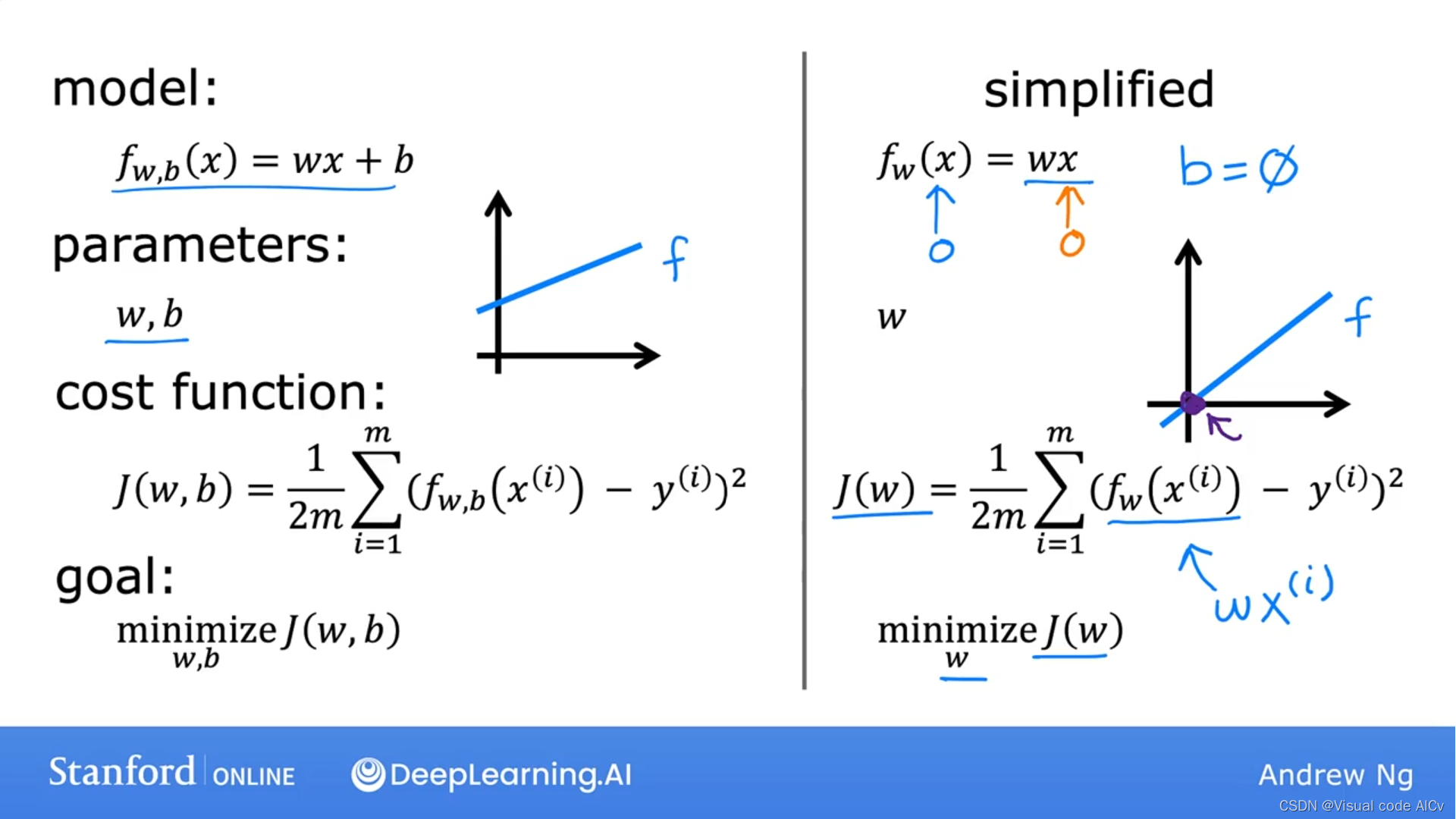
为什么均方差公式需要乘以1/2：为了方便在求导时进行计算。且乘以1/2并不会改变模型优化结果。

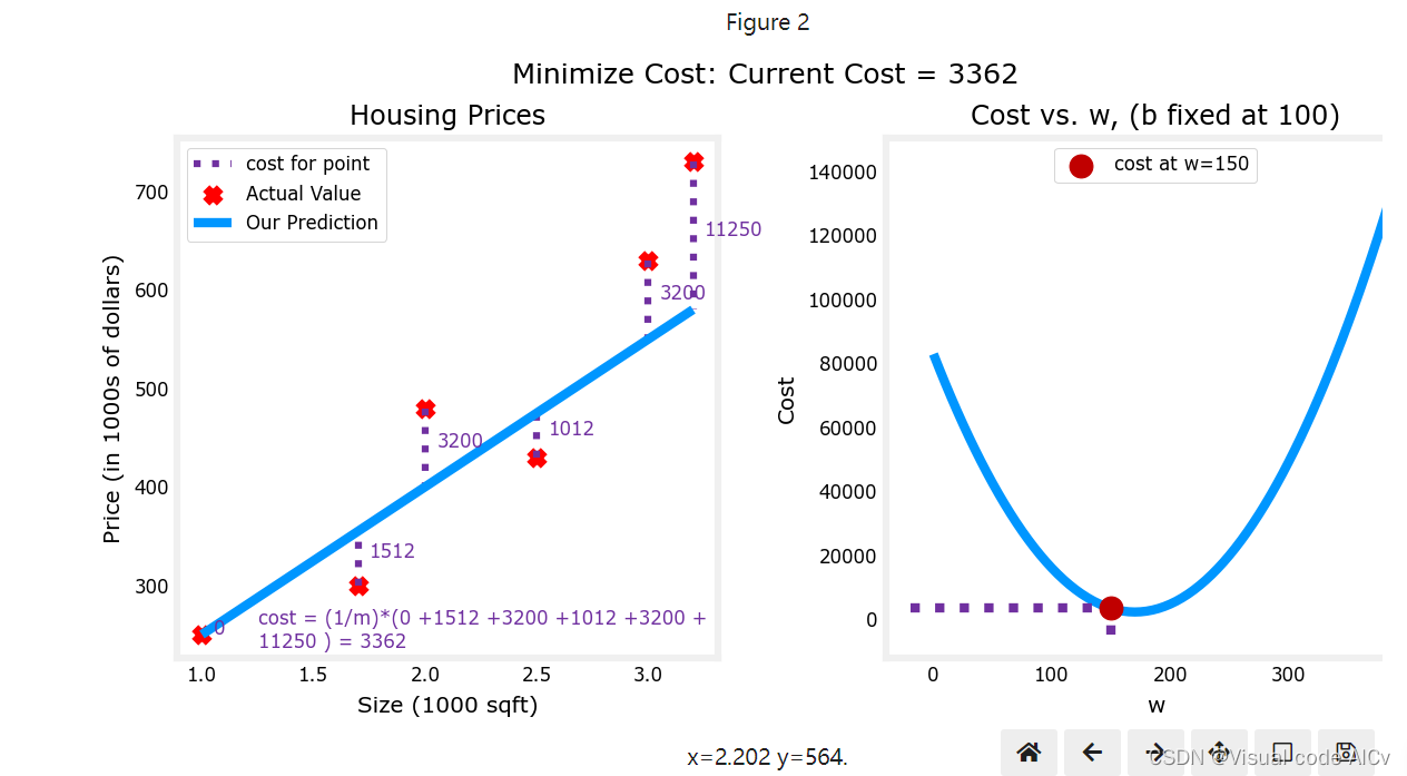
示例：

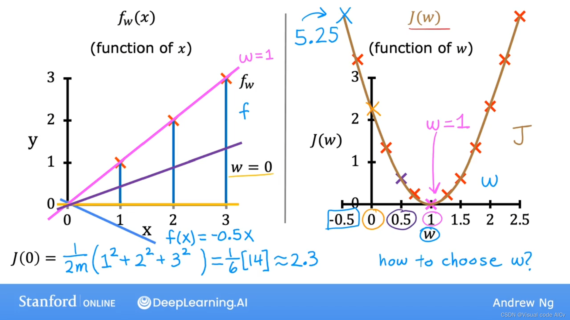
下图基于线性模型 $f_{w}(x)=wx$ ：

左图为w取不同值时 $f_{w}(x)=wx$ 对应的变化。

右图为w取不同值时对应 $J(w)$ 的变化情况。

可知当w等于1时， $J(w)$ 最小；故取w=1时，模型最优

常用损失函数：

均方误差（Mean Squared Error，MSE）：均方误差是最常见的损失函数之一，用于回归问题。它计算预测值与真实值之间的平方差的平均值。
交叉熵损失函数（Cross-Entropy Loss）：交叉熵损失函数常用于分类问题中，特别是在多类别分类问题中。它计算预测值和真实值之间的交叉熵，可以更好地反映模型对于不同类别的预测性能。
Hinge损失函数：Hinge损失函数通常用于支持向量机（SVM）中，用于最大化分类边界的间隔。
对数损失函数（Log Loss）：对数损失函数也常用于分类问题中，特别是二分类问题。它衡量预测值和真实值之间的对数差异，可以用于评估模型的分类性能。

二、均方差损失函数推导

首先，定义线性回归模型为：

$\hat{y} = \theta_0 + \theta_1x$

均方差损失函数的定义为：

$MSE = \frac{1}{2n} \sum_{i=1}^{n}(y_i - \hat{y}_i)^2$

其中，n表示样本数量，yᵢ表示真实标签，\hat{y}_i表示模型对第i个样本的预测值。

现在，我们将均方差损失函数展开：

$MSE = \frac{1}{2n} \sum_{i=1}^{n}(y_i - (\theta_0 + \theta_1x_i))^2$

我们的目标是最小化MSE，即找到使MSE最小的θ₀和θ₁。为了实现这一目标，我们可以使用梯度下降等优化算法，通过对θ₀和θ₁的偏导数进行迭代更新。

现在，我们对θ₀和θ₁分别求偏导数：

$\frac{\partial MSE}{\partial \theta_0} = \frac{1}{2n} \sum_{i=1}^{n}-2(y_i - (\theta_0 + \theta_1x_i))$

$\frac{\partial MSE}{\partial \theta_1} = \frac{1}{2n} \sum_{i=1}^{n}-2x_i(y_i - (\theta_0 + \theta_1x_i))$

接下来，我们可以使用梯度下降算法来更新θ₀和θ₁：

$\theta_0 = \theta_0 - \alpha \frac{\partial MSE}{\partial \theta_0}$

$\theta_1 = \theta_1 - \alpha \frac{\partial MSE}{\partial \theta_1}$

其中，α表示学习率，控制每次迭代的步长。

通过不断迭代更新θ₀和θ₁，直到损失函数收敛或达到预定的迭代次数，我们可以找到最优的θ₀和θ₁，从而训练出一个最优的线性回归模型。

三、损失函数可视化实例（2D）

代码来自吴恩达机器学习课程附带的资源包（~~jupyter不太会用，所以重新写一个main~~）（运行前先下载数据集[上传失败了]，还有样式）

main

import numpy as np
import matplotlib.widgets
import matplotlib.pyplot as plt
from lab_utils_uni import plt_intuition, plt_stationary, plt_update_onclick, soup_bowlplt.style.use('./deeplearning.mplstyle')x_train = np.array([1.0, 2.0])  # (size in 1000 square feet)
y_train = np.array([300.0, 500.0])def compute_cost(x, y, w, b):"""Computes the cost function for linear regression.Args:x (ndarray (m,)): Data, m examplesy (ndarray (m,)): target valuesw,b (scalar)    : model parametersReturnstotal_cost (float): The cost of using w,b as the parameters for linear regressionto fit the data points in x and y"""# number of training examplesm = x.shape[0]cost_sum = 0for i in range(m):f_wb = w * x[i] + bcost = (f_wb - y[i]) ** 2cost_sum = cost_sum + costtotal_cost = (1 / (2 * m)) * cost_sumreturn total_costplt_intuition(x_train, y_train)

lab_utils_uni.py

""" 
lab_utils_uni.pyroutines used in Course 1, Week2, labs1-3 dealing with single variables (univariate)
"""
import numpy as np
import matplotlib.pyplot as plt
from matplotlib.ticker import MaxNLocator
from matplotlib.gridspec import GridSpec
from matplotlib.colors import LinearSegmentedColormap
from ipywidgets import interact
from lab_utils_common import compute_cost
from lab_utils_common import dlblue, dlorange, dldarkred, dlmagenta, dlpurple, dlcolorsplt.style.use('./deeplearning.mplstyle')
n_bin = 5
dlcm = LinearSegmentedColormap.from_list('dl_map', dlcolors, N=n_bin)##########################################################
# Plotting Routines
##########################################################def plt_house_x(X, y,f_wb=None, ax=None):''' plot house with aXis '''if not ax:fig, ax = plt.subplots(1,1)ax.scatter(X, y, marker='x', c='r', label="Actual Value")ax.set_title("Housing Prices")ax.set_ylabel('Price (in 1000s of dollars)')ax.set_xlabel(f'Size (1000 sqft)')if f_wb is not None:ax.plot(X, f_wb,  c=dlblue, label="Our Prediction")ax.legend()def mk_cost_lines(x,y,w,b, ax):''' makes vertical cost lines'''cstr = "cost = (1/m)*("ctot = 0label = 'cost for point'addedbreak = Falsefor p in zip(x,y):f_wb_p = w*p[0]+bc_p = ((f_wb_p - p[1])**2)/2c_p_txt = c_pax.vlines(p[0], p[1],f_wb_p, lw=3, color=dlpurple, ls='dotted', label=label)label='' #just onecxy = [p[0], p[1] + (f_wb_p-p[1])/2]ax.annotate(f'{c_p_txt:0.0f}', xy=cxy, xycoords='data',color=dlpurple,xytext=(5, 0), textcoords='offset points')cstr += f"{c_p_txt:0.0f} +"if len(cstr) > 38 and addedbreak is False:cstr += "\n"addedbreak = Truectot += c_pctot = ctot/(len(x))cstr = cstr[:-1] + f") = {ctot:0.0f}"ax.text(0.15,0.02,cstr, transform=ax.transAxes, color=dlpurple)##########
# Cost lab
##########def plt_intuition(x_train, y_train):w_range = np.array([200-200,200+200])tmp_b = 100w_array = np.arange(*w_range, 5)cost = np.zeros_like(w_array)for i in range(len(w_array)):tmp_w = w_array[i]cost[i] = compute_cost(x_train, y_train, tmp_w, tmp_b)@interact(w=(*w_range,10),continuous_update=False)def func( w=150):f_wb = np.dot(x_train, w) + tmp_bfig, ax = plt.subplots(1, 2, constrained_layout=True, figsize=(8,4))fig.canvas.toolbar_position = 'bottom'mk_cost_lines(x_train, y_train, w, tmp_b, ax[0])plt_house_x(x_train, y_train, f_wb=f_wb, ax=ax[0])ax[1].plot(w_array, cost)cur_cost = compute_cost(x_train, y_train, w, tmp_b)ax[1].scatter(w,cur_cost, s=100, color=dldarkred, zorder= 10, label= f"cost at w={w}")ax[1].hlines(cur_cost, ax[1].get_xlim()[0],w, lw=4, color=dlpurple, ls='dotted')ax[1].vlines(w, ax[1].get_ylim()[0],cur_cost, lw=4, color=dlpurple, ls='dotted')ax[1].set_title("Cost vs. w, (b fixed at 100)")ax[1].set_ylabel('Cost')ax[1].set_xlabel('w')ax[1].legend(loc='upper center')fig.suptitle(f"Minimize Cost: Current Cost = {cur_cost:0.0f}", fontsize=12)plt.show()# this is the 2D cost curve with interactive slider
def plt_stationary(x_train, y_train):# setup figurefig = plt.figure( figsize=(9,8))#fig = plt.figure(constrained_layout=True,  figsize=(12,10))fig.set_facecolor('#ffffff') #whitefig.canvas.toolbar_position = 'top'#gs = GridSpec(2, 2, figure=fig, wspace = 0.01)gs = GridSpec(2, 2, figure=fig)ax0 = fig.add_subplot(gs[0, 0])ax1 = fig.add_subplot(gs[0, 1])ax2 = fig.add_subplot(gs[1, :],  projection='3d')ax = np.array([ax0,ax1,ax2])#setup useful ranges and common linspacesw_range = np.array([200-300.,200+300])b_range = np.array([50-300., 50+300])b_space  = np.linspace(*b_range, 100)w_space  = np.linspace(*w_range, 100)# get cost for w,b ranges for contour and 3Dtmp_b,tmp_w = np.meshgrid(b_space,w_space)z=np.zeros_like(tmp_b)for i in range(tmp_w.shape[0]):for j in range(tmp_w.shape[1]):z[i,j] = compute_cost(x_train, y_train, tmp_w[i][j], tmp_b[i][j] )if z[i,j] == 0: z[i,j] = 1e-6w0=200;b=-100    #initial point### plot model w cost ###f_wb = np.dot(x_train,w0) + bmk_cost_lines(x_train,y_train,w0,b,ax[0])plt_house_x(x_train, y_train, f_wb=f_wb, ax=ax[0])### plot contour ###CS = ax[1].contour(tmp_w, tmp_b, np.log(z),levels=12, linewidths=2, alpha=0.7,colors=dlcolors)ax[1].set_title('Cost(w,b)')ax[1].set_xlabel('w', fontsize=10)ax[1].set_ylabel('b', fontsize=10)ax[1].set_xlim(w_range) ; ax[1].set_ylim(b_range)cscat  = ax[1].scatter(w0,b, s=100, color=dlblue, zorder= 10, label="cost with \ncurrent w,b")chline = ax[1].hlines(b, ax[1].get_xlim()[0],w0, lw=4, color=dlpurple, ls='dotted')cvline = ax[1].vlines(w0, ax[1].get_ylim()[0],b, lw=4, color=dlpurple, ls='dotted')ax[1].text(0.5,0.95,"Click to choose w,b",  bbox=dict(facecolor='white', ec = 'black'), fontsize = 10,transform=ax[1].transAxes, verticalalignment = 'center', horizontalalignment= 'center')#Surface plot of the cost function J(w,b)ax[2].plot_surface(tmp_w, tmp_b, z,  cmap = dlcm, alpha=0.3, antialiased=True)ax[2].plot_wireframe(tmp_w, tmp_b, z, color='k', alpha=0.1)plt.xlabel("$w$")plt.ylabel("$b$")ax[2].zaxis.set_rotate_label(False)ax[2].xaxis.set_pane_color((1.0, 1.0, 1.0, 0.0))ax[2].yaxis.set_pane_color((1.0, 1.0, 1.0, 0.0))ax[2].zaxis.set_pane_color((1.0, 1.0, 1.0, 0.0))ax[2].set_zlabel("J(w, b)\n\n", rotation=90)plt.title("Cost(w,b) \n [You can rotate this figure]", size=12)ax[2].view_init(30, -120)return fig,ax, [cscat, chline, cvline]#https://matplotlib.org/stable/users/event_handling.html
class plt_update_onclick:def __init__(self, fig, ax, x_train,y_train, dyn_items):self.fig = figself.ax = axself.x_train = x_trainself.y_train = y_trainself.dyn_items = dyn_itemsself.cid = fig.canvas.mpl_connect('button_press_event', self)def __call__(self, event):if event.inaxes == self.ax[1]:ws = event.xdatabs = event.ydatacst = compute_cost(self.x_train, self.y_train, ws, bs)# clear and redraw line plotself.ax[0].clear()f_wb = np.dot(self.x_train,ws) + bsmk_cost_lines(self.x_train,self.y_train,ws,bs,self.ax[0])plt_house_x(self.x_train, self.y_train, f_wb=f_wb, ax=self.ax[0])# remove lines and re-add on countour plot and 3d plotfor artist in self.dyn_items:artist.remove()a = self.ax[1].scatter(ws,bs, s=100, color=dlblue, zorder= 10, label="cost with \ncurrent w,b")b = self.ax[1].hlines(bs, self.ax[1].get_xlim()[0],ws, lw=4, color=dlpurple, ls='dotted')c = self.ax[1].vlines(ws, self.ax[1].get_ylim()[0],bs, lw=4, color=dlpurple, ls='dotted')d = self.ax[1].annotate(f"Cost: {cst:.0f}", xy= (ws, bs), xytext = (4,4), textcoords = 'offset points',bbox=dict(facecolor='white'), size = 10)#Add point in 3D surface plote = self.ax[2].scatter3D(ws, bs,cst , marker='X', s=100)self.dyn_items = [a,b,c,d,e]self.fig.canvas.draw()def soup_bowl():""" Create figure and plot with a 3D projection"""fig = plt.figure(figsize=(8,8))#Plot configurationax = fig.add_subplot(111, projection='3d')ax.xaxis.set_pane_color((1.0, 1.0, 1.0, 0.0))ax.yaxis.set_pane_color((1.0, 1.0, 1.0, 0.0))ax.zaxis.set_pane_color((1.0, 1.0, 1.0, 0.0))ax.zaxis.set_rotate_label(False)ax.view_init(45, -120)#Useful linearspaces to give values to the parameters w and bw = np.linspace(-20, 20, 100)b = np.linspace(-20, 20, 100)#Get the z value for a bowl-shaped cost functionz=np.zeros((len(w), len(b)))j=0for x in w:i=0for y in b:z[i,j] = x**2 + y**2i+=1j+=1#Meshgrid used for plotting 3D functionsW, B = np.meshgrid(w, b)#Create the 3D surface plot of the bowl-shaped cost functionax.plot_surface(W, B, z, cmap = "Spectral_r", alpha=0.7, antialiased=False)ax.plot_wireframe(W, B, z, color='k', alpha=0.1)ax.set_xlabel("$w$")ax.set_ylabel("$b$")ax.set_zlabel("$J(w,b)$", rotation=90)ax.set_title("$J(w,b)$\n [You can rotate this figure]", size=15)plt.show()def inbounds(a,b,xlim,ylim):xlow,xhigh = xlimylow,yhigh = ylimax, ay = abx, by = bif (ax > xlow and ax < xhigh) and (bx > xlow and bx < xhigh) \and (ay > ylow and ay < yhigh) and (by > ylow and by < yhigh):return Truereturn Falsedef plt_contour_wgrad(x, y, hist, ax, w_range=[-100, 500, 5], b_range=[-500, 500, 5],contours = [0.1,50,1000,5000,10000,25000,50000],resolution=5, w_final=200, b_final=100,step=10 ):b0,w0 = np.meshgrid(np.arange(*b_range),np.arange(*w_range))z=np.zeros_like(b0)for i in range(w0.shape[0]):for j in range(w0.shape[1]):z[i][j] = compute_cost(x, y, w0[i][j], b0[i][j] )CS = ax.contour(w0, b0, z, contours, linewidths=2,colors=[dlblue, dlorange, dldarkred, dlmagenta, dlpurple])ax.clabel(CS, inline=1, fmt='%1.0f', fontsize=10)ax.set_xlabel("w");  ax.set_ylabel("b")ax.set_title('Contour plot of cost J(w,b), vs b,w with path of gradient descent')w = w_final; b=b_finalax.hlines(b, ax.get_xlim()[0],w, lw=2, color=dlpurple, ls='dotted')ax.vlines(w, ax.get_ylim()[0],b, lw=2, color=dlpurple, ls='dotted')base = hist[0]for point in hist[0::step]:edist = np.sqrt((base[0] - point[0])**2 + (base[1] - point[1])**2)if(edist > resolution or point==hist[-1]):if inbounds(point,base, ax.get_xlim(),ax.get_ylim()):plt.annotate('', xy=point, xytext=base,xycoords='data',arrowprops={'arrowstyle': '->', 'color': 'r', 'lw': 3},va='center', ha='center')base=pointreturndef plt_divergence(p_hist, J_hist, x_train,y_train):x=np.zeros(len(p_hist))y=np.zeros(len(p_hist))v=np.zeros(len(p_hist))for i in range(len(p_hist)):x[i] = p_hist[i][0]y[i] = p_hist[i][1]v[i] = J_hist[i]fig = plt.figure(figsize=(12,5))plt.subplots_adjust( wspace=0 )gs = fig.add_gridspec(1, 5)fig.suptitle(f"Cost escalates when learning rate is too large")#===============#  First subplot#===============ax = fig.add_subplot(gs[:2], )# Print w vs cost to see minimumfix_b = 100w_array = np.arange(-70000, 70000, 1000)cost = np.zeros_like(w_array)for i in range(len(w_array)):tmp_w = w_array[i]cost[i] = compute_cost(x_train, y_train, tmp_w, fix_b)ax.plot(w_array, cost)ax.plot(x,v, c=dlmagenta)ax.set_title("Cost vs w, b set to 100")ax.set_ylabel('Cost')ax.set_xlabel('w')ax.xaxis.set_major_locator(MaxNLocator(2))#===============# Second Subplot#===============tmp_b,tmp_w = np.meshgrid(np.arange(-35000, 35000, 500),np.arange(-70000, 70000, 500))z=np.zeros_like(tmp_b)for i in range(tmp_w.shape[0]):for j in range(tmp_w.shape[1]):z[i][j] = compute_cost(x_train, y_train, tmp_w[i][j], tmp_b[i][j] )ax = fig.add_subplot(gs[2:], projection='3d')ax.plot_surface(tmp_w, tmp_b, z,  alpha=0.3, color=dlblue)ax.xaxis.set_major_locator(MaxNLocator(2))ax.yaxis.set_major_locator(MaxNLocator(2))ax.set_xlabel('w', fontsize=16)ax.set_ylabel('b', fontsize=16)ax.set_zlabel('\ncost', fontsize=16)plt.title('Cost vs (b, w)')# Customize the view angleax.view_init(elev=20., azim=-65)ax.plot(x, y, v,c=dlmagenta)return# draw derivative line
# y = m*(x - x1) + y1
def add_line(dj_dx, x1, y1, d, ax):x = np.linspace(x1-d, x1+d,50)y = dj_dx*(x - x1) + y1ax.scatter(x1, y1, color=dlblue, s=50)ax.plot(x, y, '--', c=dldarkred,zorder=10, linewidth = 1)xoff = 30 if x1 == 200 else 10ax.annotate(r"$\frac{\partial J}{\partial w}$ =%d" % dj_dx, fontsize=14,xy=(x1, y1), xycoords='data',xytext=(xoff, 10), textcoords='offset points',arrowprops=dict(arrowstyle="->"),horizontalalignment='left', verticalalignment='top')def plt_gradients(x_train,y_train, f_compute_cost, f_compute_gradient):#===============#  First subplot#===============fig,ax = plt.subplots(1,2,figsize=(12,4))# Print w vs cost to see minimumfix_b = 100w_array = np.linspace(-100, 500, 50)w_array = np.linspace(0, 400, 50)cost = np.zeros_like(w_array)for i in range(len(w_array)):tmp_w = w_array[i]cost[i] = f_compute_cost(x_train, y_train, tmp_w, fix_b)ax[0].plot(w_array, cost,linewidth=1)ax[0].set_title("Cost vs w, with gradient; b set to 100")ax[0].set_ylabel('Cost')ax[0].set_xlabel('w')# plot lines for fixed b=100for tmp_w in [100,200,300]:fix_b = 100dj_dw,dj_db = f_compute_gradient(x_train, y_train, tmp_w, fix_b )j = f_compute_cost(x_train, y_train, tmp_w, fix_b)add_line(dj_dw, tmp_w, j, 30, ax[0])#===============# Second Subplot#===============tmp_b,tmp_w = np.meshgrid(np.linspace(-200, 200, 10), np.linspace(-100, 600, 10))U = np.zeros_like(tmp_w)V = np.zeros_like(tmp_b)for i in range(tmp_w.shape[0]):for j in range(tmp_w.shape[1]):U[i][j], V[i][j] = f_compute_gradient(x_train, y_train, tmp_w[i][j], tmp_b[i][j] )X = tmp_wY = tmp_bn=-2color_array = np.sqrt(((V-n)/2)**2 + ((U-n)/2)**2)ax[1].set_title('Gradient shown in quiver plot')Q = ax[1].quiver(X, Y, U, V, color_array, units='width', )ax[1].quiverkey(Q, 0.9, 0.9, 2, r'$2 \frac{m}{s}$', labelpos='E',coordinates='figure')ax[1].set_xlabel("w"); ax[1].set_ylabel("b")

lab_utils_common.py

""" 
lab_utils_common.pyfunctions common to all optional labs, Course 1, Week 2 
"""import numpy as np
import matplotlib.pyplot as pltplt.style.use('./deeplearning.mplstyle')
dlblue = '#0096ff'; dlorange = '#FF9300'; dldarkred='#C00000'; dlmagenta='#FF40FF'; dlpurple='#7030A0';
dlcolors = [dlblue, dlorange, dldarkred, dlmagenta, dlpurple]
dlc = dict(dlblue = '#0096ff', dlorange = '#FF9300', dldarkred='#C00000', dlmagenta='#FF40FF', dlpurple='#7030A0')##########################################################
# Regression Routines
###########################################################Function to calculate the cost
def compute_cost_matrix(X, y, w, b, verbose=False):"""Computes the gradient for linear regressionArgs:X (ndarray (m,n)): Data, m examples with n featuresy (ndarray (m,)) : target valuesw (ndarray (n,)) : model parameters  b (scalar)       : model parameterverbose : (Boolean) If true, print out intermediate value f_wbReturnscost: (scalar)"""m = X.shape[0]# calculate f_wb for all examples.f_wb = X @ w + b# calculate costtotal_cost = (1/(2*m)) * np.sum((f_wb-y)**2)if verbose: print("f_wb:")if verbose: print(f_wb)return total_costdef compute_gradient_matrix(X, y, w, b):"""Computes the gradient for linear regressionArgs:X (ndarray (m,n)): Data, m examples with n featuresy (ndarray (m,)) : target valuesw (ndarray (n,)) : model parameters  b (scalar)       : model parameterReturnsdj_dw (ndarray (n,1)): The gradient of the cost w.r.t. the parameters w.dj_db (scalar):        The gradient of the cost w.r.t. the parameter b."""m,n = X.shapef_wb = X @ w + be   = f_wb - ydj_dw  = (1/m) * (X.T @ e)dj_db  = (1/m) * np.sum(e)return dj_db,dj_dw# Loop version of multi-variable compute_cost
def compute_cost(X, y, w, b):"""compute costArgs:X (ndarray (m,n)): Data, m examples with n featuresy (ndarray (m,)) : target valuesw (ndarray (n,)) : model parameters  b (scalar)       : model parameterReturnscost (scalar)    : cost"""m = X.shape[0]cost = 0.0for i in range(m):f_wb_i = np.dot(X[i],w) + b           #(n,)(n,)=scalarcost = cost + (f_wb_i - y[i])**2cost = cost/(2*m)return cost def compute_gradient(X, y, w, b):"""Computes the gradient for linear regressionArgs:X (ndarray (m,n)): Data, m examples with n featuresy (ndarray (m,)) : target valuesw (ndarray (n,)) : model parameters  b (scalar)       : model parameterReturnsdj_dw (ndarray Shape (n,)): The gradient of the cost w.r.t. the parameters w.dj_db (scalar):             The gradient of the cost w.r.t. the parameter b."""m,n = X.shape           #(number of examples, number of features)dj_dw = np.zeros((n,))dj_db = 0.for i in range(m):err = (np.dot(X[i], w) + b) - y[i]for j in range(n):dj_dw[j] = dj_dw[j] + err * X[i,j]dj_db = dj_db + errdj_dw = dj_dw/mdj_db = dj_db/mreturn dj_db,dj_dw

效果