【GNN2】PyG完成图分类任务，新手入门，保姆级教程-编程知识

上次讲了如何给节点分类，这次我们来看如何用GNN完成图分类任务，也就是Graph-level的任务。

【GNN 1】PyG实现图神经网络，完成节点分类任务，人话、保姆级教程-CSDN博客

图分类就是以图为单位的分类，举个例子：每个学校都有社交关系网，图分类就是通过这个社交网络判别这个学校是小学、初中、高中还是大学。

实现方法就是通过利用图的结构信息，对图进行嵌入（embed），也就是用向量来表示这个图，使得分类器基于这个向量能够轻松分类，或者说通过对图进行向量表示，使得图的分类尽可能变成一个线性可分的任务。

下图就是形象展示了我们要干的事：把一堆图表示成线性可分的向量们，然后构建个分类器，完成图分类。

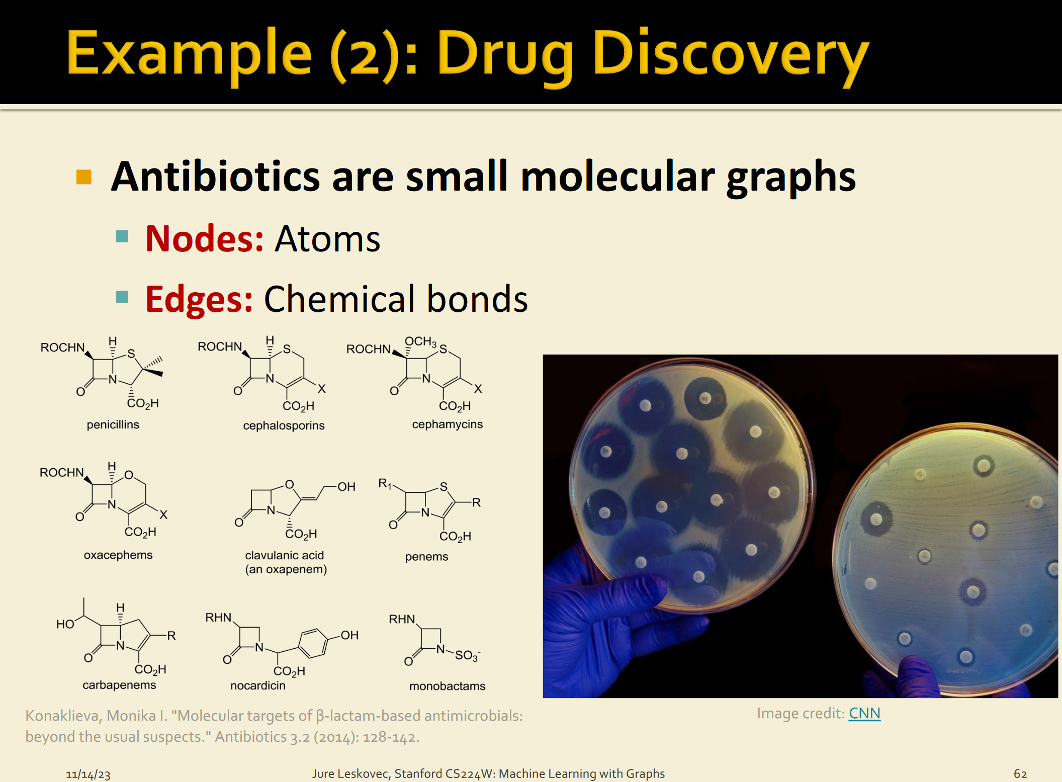
图分类的一个经典任务就是分子属性预测，我们可以把原子看成图的节点，化学键看成边，整个分子就是图，我们想知道分子有什么性质（是否是药物小分子，能否和蛋白相互作用等），其实就是看这个图是属于哪一个类别的。

数据集的选择

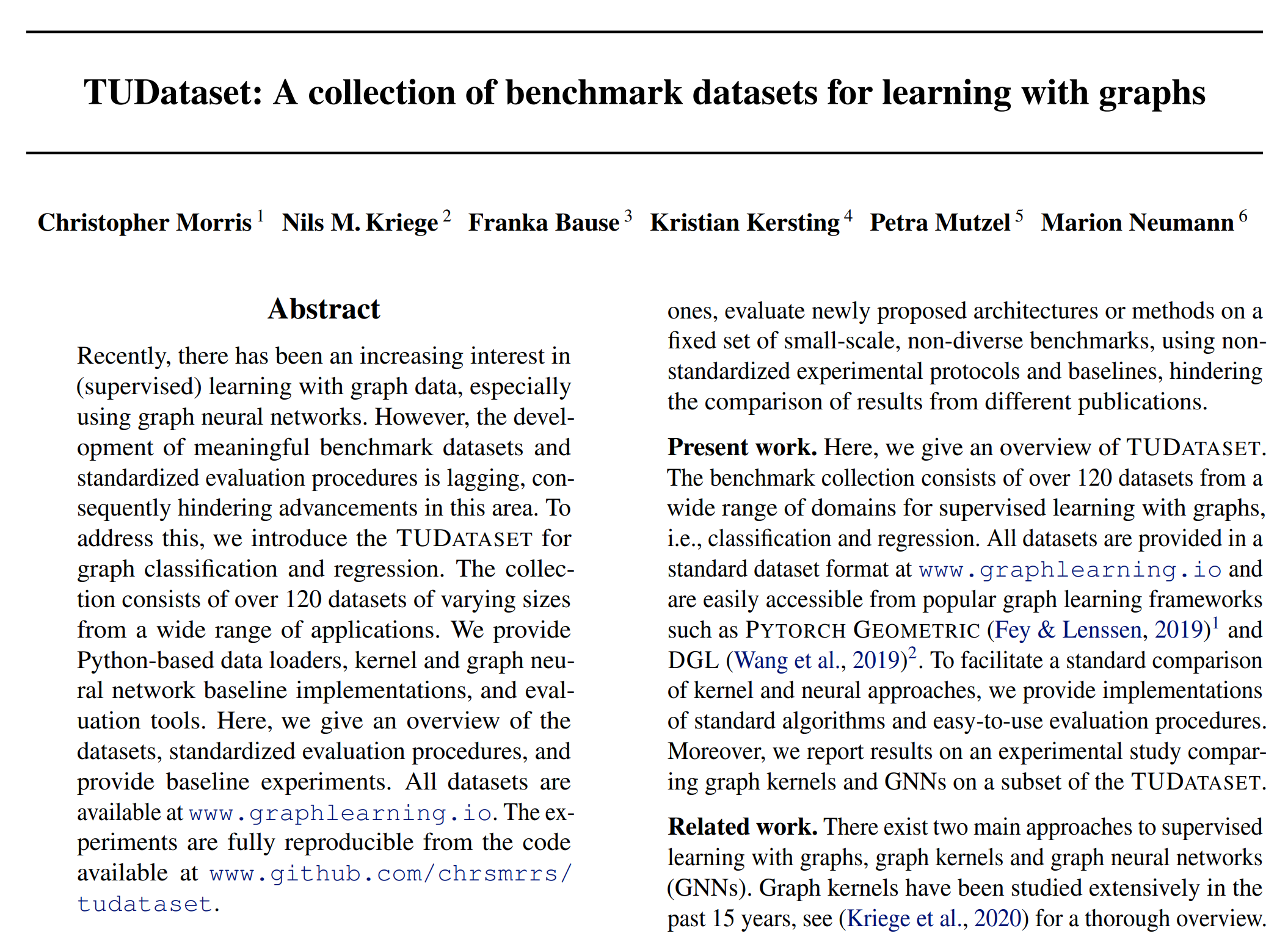
我们这次选择的数据集是TUDatasets，这是TU Dortumnd University收集的大量关于分子特征的图数据，他们还发表了论文TUDataset: A collection of benchmark datasets for learning with graphs。

这么重要的数据集，当然也可以通过PyTorch Geometric直接加载啦。

下面是数据集的大致情况，可以看到这里包括酶、蛋白质还有其他的一些。注意了第一列不是第二列的类别，最后一列class才是。

加载数据

下面我们来加载数据吧！

先说一下TUDataset这个函数，有两个参数，

root (str) – Root directory where the dataset should be saved.（保存的路径）
name (str) – The name of the dataset.（名字）

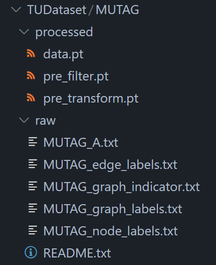
加载完就可以发现数据已经下载到我们指定的root目录了。

# Install required packages.
import os
import torch
os.environ['TORCH'] = torch.__version__
print(torch.__version__)# !pip install -q torch-scatter -f https://data.pyg.org/whl/torch-${TORCH}.html
# !pip install -q torch-sparse -f https://data.pyg.org/whl/torch-${TORCH}.html
# !pip install -q git+https://github.com/pyg-team/pytorch_geometric.gitimport torch
from torch_geometric.datasets import TUDatasetdataset = TUDataset(root='data/TUDataset', name='MUTAG')
# - root (str) – Root directory where the dataset should be saved.（保存的路径）
# - name (str) – The name of the dataset.（名字）# 查看一些数据集的基本信息
print()
print(f'Dataset: {dataset}:')
print('====================')
print(f'Number of graphs: {len(dataset)}')
print(f'Number of features: {dataset.num_features}')
print(f'Number of classes: {dataset.num_classes}')data = dataset[0]  # Get the first graph object.print()
print(data)
print('=============================================================')# 看一下第一张图的信息
# Gather some statistics about the first graph.
print(f'Number of nodes: {data.num_nodes}')
print(f'Number of edges: {data.num_edges}')
print(f'Average node degree: {data.num_edges / data.num_nodes:.2f}')
print(f'Has isolated nodes: {data.has_isolated_nodes()}')
print(f'Has self-loops: {data.has_self_loops()}')
print(f'Is undirected: {data.is_undirected()}')

Dataset: MUTAG(188):
====================
Number of graphs: 188
Number of features: 7
Number of classes: 2Data(edge_index=[2, 38], x=[17, 7], edge_attr=[38, 4], y=[1])
=============================================================
Number of nodes: 17
Number of edges: 38
Average node degree: 2.24
Has isolated nodes: False
Has self-loops: False
Is undirected: True

这个数据集有188张图，有两个类。

通过查看第一个图的基本信息，我们可以看到它有17个节点（7维特征向量，用一个7维的向量来描述节点）、38条无向边（4维特征向量，用一个4维的向量给来描述边，因为是入门，这次我们不用）还有一个图的标签y=[1]表示图是哪一类的（1维向量，一个数）。

这里提一个小知识点，在机器学习中，训练之前一般均会对数据集做shuffle，也就是打乱数据之间的顺序，让数据随机化，这样可以避免过拟合。

数据集shuffle的重要性 - 知乎 (zhihu.com)

PyTorch Geometric也提供了很多处理图数据集的方法，比如shuffle()，我们今天就首先对数据集进行打乱，然后选择前150个样本进行训练，剩下的38个进行测试。

torch.manual_seed(12345)
dataset = dataset.shuffle()train_dataset = dataset[:150]
test_dataset = dataset[150:]print(f'Number of training graphs: {len(train_dataset)}')
print(f'Number of test graphs: {len(test_dataset)}')

Number of training graphs: 150
Number of test graphs: 38

图的Mini-batching

因为在图分类数据集中的图通常来说都比较小，这样就不能充分利用GPU，所以一个想法就是就是先batch the graph，然后再把图放到GNN中。

在图像和自然语言处理领域，这个过程通常是通过rescaling或者padding来实现的，就是把每个样本转换成统一大小/形状，然后再把它们放到一起。以图片为例，我把所有图片都转换为100*100大小，然后再把这些图像融合成一个大图（或者以其他形式存储），这个存储的变量也是有维度的，这个维度的大小就是在一个batch中样本的个数，也就是batch size。

在GNN中，rescaling和padding要么行不通，要么会造成不必要的内存消耗。

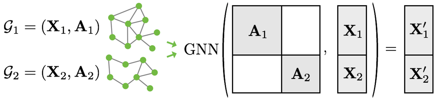
因此，PyTorch Geometric选择了另一种方法来实现多个样本的并行化。在这里，邻接矩阵以对角线方式堆叠(创建一个包含多个孤立子图的大图，A)，node和target特征在节点维度上简单地拼接起来（X）:

这个过程相对于其他的batching方法有一些关键的优势：

依赖于消息传递方案（message passing scheme）的GNN operators不需要修改，因为消息不会在属于不同图的两个节点之间交换；
没有计算或内存开销，因为邻接矩阵以稀疏矩阵的方式保存，只保存非零条目，也就是只保留边。

PyTorch Geometric在torch_geometrics .data. dataloader类的帮助下自动处理将多个图批处理为一个大图（batching multiple graphs into a single giant graph）:

from torch_geometric.loader import DataLoadertrain_loader = DataLoader(train_dataset, batch_size=64, shuffle=True)
test_loader = DataLoader(test_dataset, batch_size=64, shuffle=False)for step, data in enumerate(train_loader):print(f'Step {step + 1}:')print('=======')print(f'Number of graphs in the current batch: {data.num_graphs}')print(data)print()for step, data in enumerate(test_loader):print(f'Step {step + 1}:')print('=======')print(f'Number of graphs in the current batch: {data.num_graphs}')print(data)print()

Step 1:
=======
Number of graphs in the current batch: 64
DataBatch(edge_index=[2, 2572], x=[1168, 7], edge_attr=[2572, 4], y=[64], batch=[1168], ptr=[65])Step 2:
=======
Number of graphs in the current batch: 64
DataBatch(edge_index=[2, 2554], x=[1153, 7], edge_attr=[2554, 4], y=[64], batch=[1153], ptr=[65])Step 3:
=======
Number of graphs in the current batch: 22
DataBatch(edge_index=[2, 868], x=[393, 7], edge_attr=[868, 4], y=[22], batch=[393], ptr=[23])Step 1:
=======
Number of graphs in the current batch: 38
DataBatch(edge_index=[2, 1448], x=[657, 7], edge_attr=[1448, 4], y=[38], batch=[657], ptr=[39])

我们选择将batch_size设置为64，可以看到分成了3个随机打乱的mini-batches。

对于每个 Batch对象都有一个对应的batch vector，这就是起到一个索引的作用，即将每个节点映射到batch中各自的图上。

$\textrm{batch} = [ 0, \ldots, 0, 1, \ldots, 1, 2, \ldots ]$

训练GNN

图分类任务的GNN训练一般是这样的流程：

通过几次信息传递（message passing）对每个节点进行嵌入
把节点嵌入聚合成图嵌入（readout layer）
根据图嵌入向量训练最终的分类器

有很多论文开发了很多readout层，不过其实用的最多的还是直接把节点嵌入求平均：

$\mathbf{x}_{\mathcal{G}} = \frac{1}{|\mathcal{V}|} \sum_{v \in \mathcal{V}} \mathcal{x}^{(L)}_v$

PyTorch Geometric提供了torch_geometric.nn.global_mean_pool这个函数。输入：①mini batch中所有node的embeddings；②分配向量batch；输出：每个batch中每个图经过计算得到的graph embedding，大小是 [batch_size, hidden_channels]

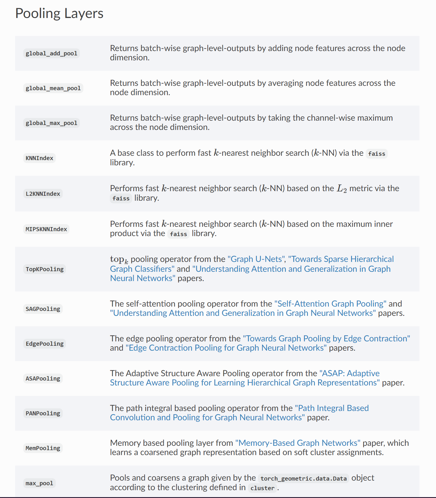
还有很多其他的pooling函数，之后会试试的。

完整的架构我们直接通过print(model)就可以看到，这个模型可以实现端到端的图分类了！

from torch.nn import Linear
import torch.nn.functional as F
from torch_geometric.nn import GCNConv
from torch_geometric.nn import global_mean_poolclass GCN(torch.nn.Module):def __init__(self, hidden_channels):super(GCN, self).__init__()torch.manual_seed(12345)self.conv1 = GCNConv(dataset.num_node_features, hidden_channels)self.conv2 = GCNConv(hidden_channels, hidden_channels)self.conv3 = GCNConv(hidden_channels, hidden_channels)self.lin = Linear(hidden_channels, dataset.num_classes)def forward(self, x, edge_index, batch):# 1. Obtain node embeddingsx = self.conv1(x, edge_index)x = x.relu()x = self.conv2(x, edge_index)x = x.relu()x = self.conv3(x, edge_index)# 2. Readout layerx = global_mean_pool(x, batch)  # [batch_size, hidden_channels]# 3. Apply a final classifierx = F.dropout(x, p=0.5, training=self.training)x = self.lin(x)return xmodel = GCN(hidden_channels=64)
print(model)

GCN((conv1): GCNConv(7, 64)(conv2): GCNConv(64, 64)(conv3): GCNConv(64, 64)(lin): Linear(in_features=64, out_features=2, bias=True)
)

我们为GCN层选择的激活函数是 $\mathrm{ReLU}(x) = \max(x, 0)$ （除了最后的readout layer）。

让我们训练一下我们的模型吧，看看它在测试集上表现如何！

from IPython.display import Javascript
display(Javascript('''google.colab.output.setIframeHeight(0, true, {maxHeight: 300})'''))model = GCN(hidden_channels=64)
# 模型的核心，64个hidden_channels，类似于神经网络的隐藏层的神经元个数
optimizer = torch.optim.Adam(model.parameters(), lr=0.01)
criterion = torch.nn.CrossEntropyLoss()def train():model.train()# 把模型设置为训练模式for data in train_loader:  # Iterate in batches over the training dataset.out = model(data.x, data.edge_index, data.batch)  # Perform a single forward pass.loss = criterion(out, data.y)  # Compute the loss.loss.backward()  # Derive gradients.#  计算梯度optimizer.step()  # Update parameters based on gradients.#  根据上面计算的梯度更新参数optimizer.zero_grad()  # Clear gradients.#  清除梯度，为下一个批次的数据做准备，相当于从头开始def test(loader):model.eval()# 把模型设置为评估模式correct = 0#  初始化correct为0，表示预测对的个数for data in loader:  # Iterate in batches over the training/test dataset.out = model(data.x, data.edge_index, data.batch)#  预测的输出值pred = out.argmax(dim=1)  # Use the class with highest probability.#  每个类别对应一个概率，概率最大的就是对应的预测值correct += int((pred == data.y).sum())  # Check against ground-truth labels.#  如果一样，就是True，也就是1，correct就+1# 准确率就是正确的/总的return correct / len(loader.dataset)  # Derive ratio of correct predictions.for epoch in range(1, 171):train()train_acc = test(train_loader)test_acc = test(test_loader)print(f'Epoch: {epoch:03d}, Train Acc: {train_acc:.4f}, Test Acc: {test_acc:.4f}')

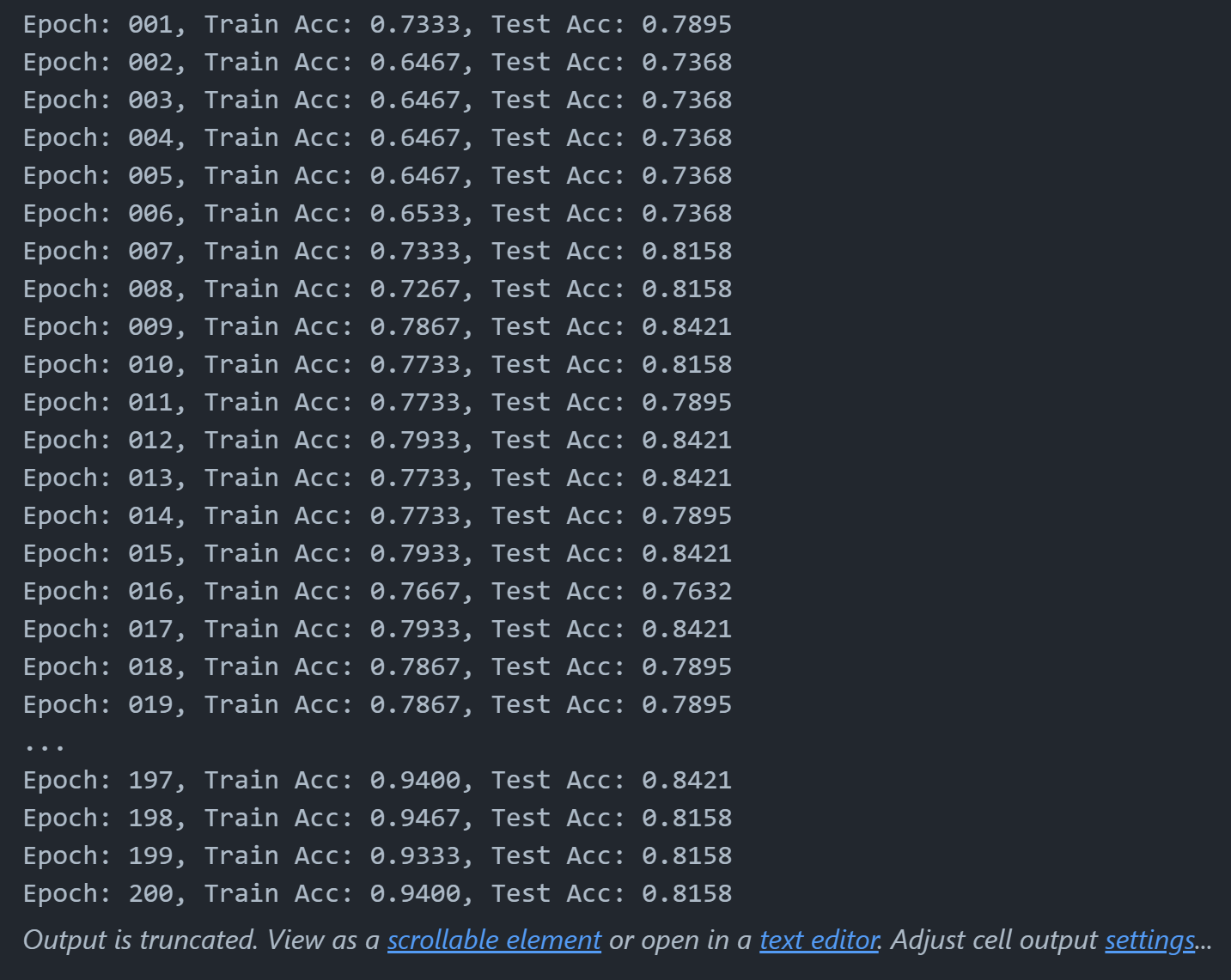
可以看到，我们的模型有0.76的测试集准确度。

波动的原因可以认为是测试集太小了，通常来说，如果数据集比较大这种波动情况就会消失。

换个架构看看效果怎么样

我们可以做的更好吗？当然可以。

正如多篇论文指出的那样(Xu et al. (2018)， Morris et al. (2018))，应用邻域归一化降低了gnn在识别某些图结构方面的表达能力（neighborhood normalization decrease the expressivity of GNNs in distingushiing certain graph structures）。

另一种替代公式（ Morris et al. (2018)）完全省略了邻域归一化，并在GNN层中添加了一个简单的跳过连接，以保留中心节点信息:
$\mathbf{x}_v^{(\ell+1)} = \mathbf{W}^{(\ell + 1)}_1 \mathbf{x}_v^{(\ell)} + \mathbf{W}^{(\ell + 1)}_2 \sum_{w \in \mathcal{N}(v)} \mathbf{x}_w^{(\ell)}$

这个layer也可以在PyG中轻松调用，也就是GraphConv。

也就是说，我们想用PyG’s GraphConv 而不是 GCNConv，然后看看效果怎么样。

from torch_geometric.nn import GraphConvclass GNN(torch.nn.Module):def __init__(self, hidden_channels):super(GNN, self).__init__()torch.manual_seed(12345)self.conv1 = GraphConv(dataset.num_node_features, hidden_channels)  # TODOself.conv2 = GraphConv(hidden_channels, hidden_channels)  # TODOself.conv3 = GraphConv(hidden_channels, hidden_channels)  # TODOself.lin = Linear(hidden_channels, dataset.num_classes)def forward(self, x, edge_index, batch):x = self.conv1(x, edge_index)x = x.relu()x = self.conv2(x, edge_index)x = x.relu()x = self.conv3(x, edge_index)x = global_mean_pool(x, batch)x = F.dropout(x, p=0.5, training=self.training)x = self.lin(x)return xmodel = GNN(hidden_channels=64)
print(model)

GNN((conv1): GraphConv(7, 64)(conv2): GraphConv(64, 64)(conv3): GraphConv(64, 64)(lin): Linear(in_features=64, out_features=2, bias=True)
)

from IPython.display import Javascript
display(Javascript('''google.colab.output.setIframeHeight(0, true, {maxHeight: 300})'''))model = GNN(hidden_channels=64)
print(model)
optimizer = torch.optim.Adam(model.parameters(), lr=0.01)for epoch in range(1, 201):train()train_acc = test(train_loader)test_acc = test(test_loader)print(f'Epoch: {epoch:03d}, Train Acc: {train_acc:.4f}, Test Acc: {test_acc:.4f}')

GNN((conv1): GraphConv(7, 64)(conv2): GraphConv(64, 64)(conv3): GraphConv(64, 64)(lin): Linear(in_features=64, out_features=2, bias=True)
)

总结

我们学习了如何应用GNN完成图分类，调用了GraphConv和GCNConv两种架构，举一反三，之后想用什么layer就用什么layer。

此外我们还学习了如何让单个的图组成batch，从而更好地利用GPU，以及如何应用readout layer从node embedding中得到graph embedding。

参考资料：

3. Graph Classification.ipynb - Colaboratory (google.com)

Colab Notebooks and Video Tutorials — pytorch_geometric documentation (pytorch-geometric.readthedocs.io)

如果觉得还不错，记得点赞+收藏哟！谢谢大家的阅读！（￣︶￣）↗