🧡🧡实验内容🧡🧡
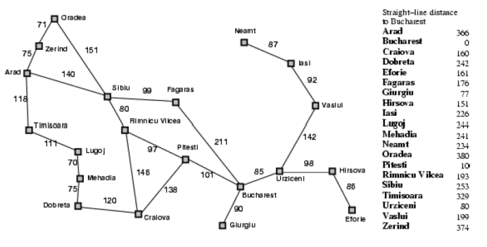
根据上图以Zerind为初始状态,Bucharest为目标状态实现搜索,分别以贪婪搜索(只考虑直线距离)和A算法求解最短路径。 按顺序列出贪婪算法探索的扩展节点和其估价函数值,A算法探索的扩展节点和其估计值。
🧡🧡相关数据结构定义🧡🧡
状态表示的数据结构
每个城市代表一个状态,每个状态的属性主要包括:
- 当前城市可从哪里来
- 从起点到当前城市总花费的实际代价(代价函数g(x))
- 当前城市到终点的直线距离(启发函数h(x))
-

状态扩展规则的表示
定义实际距离:
主要是根据设定好的字典类型的变量,选择下一个城市,如下,例如Arad城市可以到达Zerind、Sibiu、Timisoara,后面数值为Arad到达它们的实际路程(也即图中线段上的数值)。

定义理想直线距离
直接用字典表示即可

🧡🧡贪婪搜索求解🧡🧡
思想
首先了解估价函数f (x)=g(x)+h(x) 中,
- f(x)为估价函数
- g(x)为代价函数,代表从起点到当前x点的所花费的代价(距离)
- h(x)为启发函数,代表当前x点到终点的估计代价(距离)
当 不采用h(x)即g(x)=0时,f(x)=h(x),此时搜索为贪婪搜索,即每一次扩展均选择与终点离得最近(本题中h(x)为两城市的直线理想距离,而非线段上的真实距离)的城市
代码
# 贪婪搜索
import queueclass GBFS:def __init__(self, graph, heuristic, start, goal):self.graph = graph # 图self.heuristic = heuristic # 启发函数hnself.start = start # 起点self.goal = goal # 终点self.came_from = {} # 记录每个城市可以从哪里来(父节点)self.cost_so_far = {} # 从起点到该点总共花费的实际代价# 输出路径 和 对应的估计函数值def __show_path(self):current = self.goalpath = [current] # 先导入终点citywhile current != self.start: # 从终点回溯到起点city,加入所经citycurrent = self.came_from[current]path.append(current)path = path[::-1]for i in range(len(path)-1):#\033[1;91m.....\033[0m为红色加粗的ANSI转义码print(f"=====================↓↓↓cur city: \033[1;91m{path[i]}\033[0m↓↓↓=====================") for can_to_city in self.graph[path[i]].keys():print(f"can_to_city: \033[94m{can_to_city}\033[0m\t\t fn=\033[1;93m{self.heuristic[can_to_city]}\033[0m")print(f"选择fn最小的city: \033[1;92m{path[i+1]}\033[0m\n")def solve(self):frontier = queue.PriorityQueue()frontier.put((0, self.start)) # 将起点优先级设置为0,越小越优先self.came_from[self.start] = None # 父节点self.cost_so_far[self.start] = 0 # 从起点到cur city总共花费的fnclose_=[]open_=[self.start]while not frontier.empty():current = frontier.get()[1]# 打印open_和close_表
# print(f"open: {open_} \nclose: {close_} \n")
# open_.extend(list(self.graph[current].keys()))
# open_.remove(current)
# close_.append(current)if current == self.goal:self.__show_path()breakfor next in self.graph[current]: # 遍历current city 的next citynew_cost = self.cost_so_far[current] + self.heuristic[next]if next not in self.cost_so_far or new_cost < self.cost_so_far[next]:self.cost_so_far[next] = new_costpriority = new_costfrontier.put((priority, next))self.came_from[next] = current# 定义罗马尼亚地图
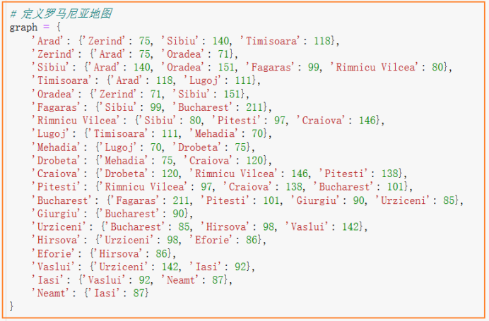
graph = {'Arad': {'Zerind': 75, 'Sibiu': 140, 'Timisoara': 118},'Zerind': {'Arad': 75, 'Oradea': 71},'Sibiu': {'Arad': 140, 'Oradea': 151, 'Fagaras': 99, 'Rimnicu Vilcea': 80},'Timisoara': {'Arad': 118, 'Lugoj': 111},'Oradea': {'Zerind': 71, 'Sibiu': 151},'Fagaras': {'Sibiu': 99, 'Bucharest': 211},'Rimnicu Vilcea': {'Sibiu': 80, 'Pitesti': 97, 'Craiova': 146},'Lugoj': {'Timisoara': 111, 'Mehadia': 70},'Mehadia': {'Lugoj': 70, 'Drobeta': 75},'Drobeta': {'Mehadia': 75, 'Craiova': 120},'Craiova': {'Drobeta': 120, 'Rimnicu Vilcea': 146, 'Pitesti': 138},'Pitesti': {'Rimnicu Vilcea': 97, 'Craiova': 138, 'Bucharest': 101},'Bucharest': {'Fagaras': 211, 'Pitesti': 101, 'Giurgiu': 90, 'Urziceni': 85},'Giurgiu': {'Bucharest': 90},'Urziceni': {'Bucharest': 85, 'Hirsova': 98, 'Vaslui': 142},'Hirsova': {'Urziceni': 98, 'Eforie': 86},'Eforie': {'Hirsova': 86},'Vaslui': {'Urziceni': 142, 'Iasi': 92},'Iasi': {'Vaslui': 92, 'Neamt': 87},'Neamt': {'Iasi': 87}
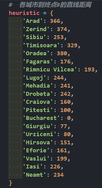
}# 各城市到终点B的直线距离
heuristic = {'Arad': 366,'Zerind': 374,'Sibiu': 253,'Timisoara': 329,'Oradea': 380,'Fagaras': 176,'Rimnicu Vilcea': 193,'Lugoj': 244,'Mehadia': 241,'Drobeta': 242,'Craiova': 160,'Pitesti': 100,'Bucharest': 0,'Giurgiu': 77,'Urziceni': 80,'Hirsova': 151,'Eforie': 161,'Vaslui': 199,'Iasi': 226,'Neamt': 234
}start = 'Zerind'
goal = 'Bucharest'gbfs = GBFS(graph, heuristic, start, goal)
gbfs.solve()运行结果
每次均选择h(x)(理想直线距离)小的城市,最终得出通过贪婪搜索算法搜出的最短路径为Zerind–>Arad–>Sibiu–>Fagaras

🧡🧡A*搜索求解🧡🧡
思想
估价函数:f(x) = g(x) + h(x)
即每一次扩展时,除了考虑选择离终点最近(直线距离h(x))的城市外,还考虑从起点城市到当前城市的实际距离(路段的真实权值g(x))
代码
# A*
import queueclass A_search:def __init__(self, graph, heuristic, start, goal):self.graph = graph # 图self.heuristic = heuristic # 启发函数hnself.start = start # 起点self.goal = goal # 终点self.came_from = {} # 记录每个城市可以从哪里来(父节点)self.cost_so_far = {} # 从起点到该点总共花费的实际代价# 输出路径 和 对应的估计函数值def __show_path(self):current = self.goalpath = [current] # 先导入终点citywhile current != self.start: # 从终点回溯到起点city,加入所经citycurrent = self.came_from[current]path.append(current)path = path[::-1]for i in range(len(path)-1):#\033[1;91m.....\033[0m为红色加粗的ANSI转义码print(f"=====================↓↓↓cur city: \033[1;91m{path[i]}\033[0m↓↓↓=====================") for can_to_city,cost in self.graph[path[i]].items():gn=self.cost_so_far[path[i]] # 起点到cur city的实际代价c=cost # cur city到next city的路途权值hn=self.heuristic[can_to_city] # next city到终点的直线距离fn=gn+c+hnprint(f"can_to_city: \033[94m{can_to_city}\033[0m\t\t fn={gn}+{c}+{hn}=\033[1;93m{fn}\033[0m")print(f"选择fn最小的city: \033[1;92m{path[i+1]}\033[0m\n")def solve(self):frontier = queue.PriorityQueue()frontier.put((0, self.start)) # 将起点优先级设置为0,越小越优先self.came_from[self.start] = None # 父节点self.cost_so_far[self.start] = 0 # 从起点到该点总共花费的fnclose_=[]open_=[self.start]while not frontier.empty():current = frontier.get()[1]# 打印open_和close_表
# print(f"open: {open_} \nclose: {close_} \n")
# open_.extend(list(self.graph[current].keys()))
# open_.remove(current)
# close_.append(current)if current == self.goal:self.__show_path()breakfor next in self.graph[current]: # 遍历current city 的next citynew_cost = self.cost_so_far[current] + self.graph[current][next] # 实际代价if next not in self.cost_so_far or new_cost < self.cost_so_far[next]:self.cost_so_far[next] = new_costpriority = new_cost + self.heuristic[next] # 修改优先级为实际代价加上启发式函数值frontier.put((priority, next))self.came_from[next] = current# 定义罗马尼亚地图
graph = {'Arad': {'Zerind': 75, 'Sibiu': 140, 'Timisoara': 118},'Zerind': {'Arad': 75, 'Oradea': 71},'Sibiu': {'Arad': 140, 'Oradea': 151, 'Fagaras': 99, 'Rimnicu Vilcea': 80},'Timisoara': {'Arad': 118, 'Lugoj': 111},'Oradea': {'Zerind': 71, 'Sibiu': 151},'Fagaras': {'Sibiu': 99, 'Bucharest': 211},'Rimnicu Vilcea': {'Sibiu': 80, 'Pitesti': 97, 'Craiova': 146},'Lugoj': {'Timisoara': 111, 'Mehadia': 70},'Mehadia': {'Lugoj': 70, 'Drobeta': 75},'Drobeta': {'Mehadia': 75, 'Craiova': 120},'Craiova': {'Drobeta': 120, 'Rimnicu Vilcea': 146, 'Pitesti': 138},'Pitesti': {'Rimnicu Vilcea': 97, 'Craiova': 138, 'Bucharest': 101},'Bucharest': {'Fagaras': 211, 'Pitesti': 101, 'Giurgiu': 90, 'Urziceni': 85},'Giurgiu': {'Bucharest': 90},'Urziceni': {'Bucharest': 85, 'Hirsova': 98, 'Vaslui': 142},'Hirsova': {'Urziceni': 98, 'Eforie': 86},'Eforie': {'Hirsova': 86},'Vaslui': {'Urziceni': 142, 'Iasi': 92},'Iasi': {'Vaslui': 92, 'Neamt': 87},'Neamt': {'Iasi': 87}
}# 各城市到终点B的直线距离
heuristic = {'Arad': 366,'Zerind': 374,'Sibiu': 253,'Timisoara': 329,'Oradea': 380,'Fagaras': 176,'Rimnicu Vilcea': 192,'Lugoj': 244,'Mehadia': 241,'Drobeta': 242,'Craiova': 160,'Pitesti': 100,'Bucharest': 0,'Giurgiu': 77,'Urziceni': 80,'Hirsova': 151,'Eforie': 161,'Vaslui': 199,'Iasi': 226,'Neamt': 234
}start = 'Zerind'
goal = 'Bucharest'a = A_search(graph, heuristic, start, goal)
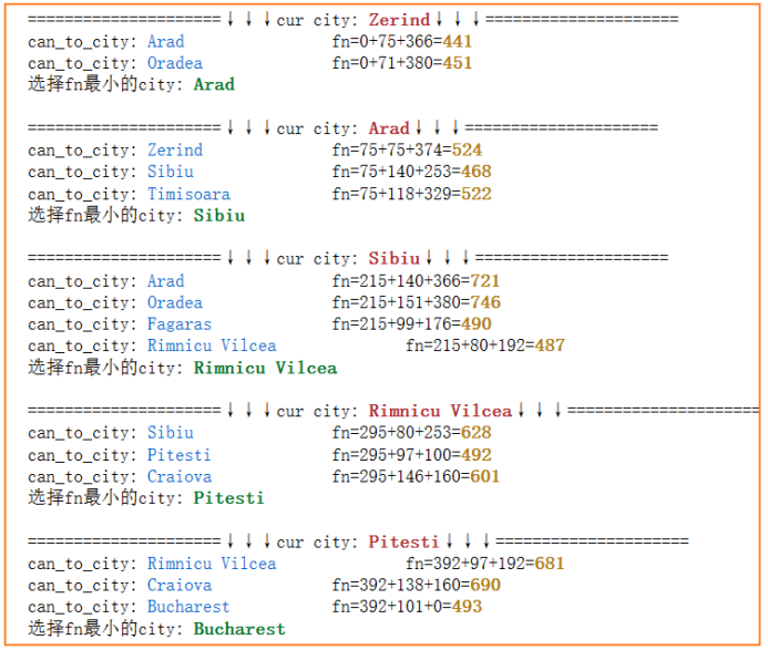
a.solve()运行结果
每次考虑已花费的代价g和未来的估计代价h
解释一下 f 的计算
当前城市为Zerind时,到达Arad的估价代价f(Arad)=g(Arad)+h(Arad),而其中g(Arad)=g(Zerind)+cost(Zerind,Arad),因此f(Arad)=g(Zerind)+cost(Zerind,Arad)+h(Arad),又因为是起点,所以g(Zerind)为0。其中:g(Zerind)为到达Zerind已经走过的距离,cost(Zerind,Arad)为图中线段权值,即Zerind到Arad的实际距离,h(Arad)为Arad到终点的理想直线距离(上面的路径图中右侧的表格),同理对于城市Oradea也是一样的计算。
当前城市为Arad时,这里没有设置close表,因此它仍然可以选择返回到Zerind,这时由城市Arad到达Zerind城市的估计代价为 f(Zerind)=g(Zerind)+h(Zerind)=g(Arad)+cost(Arad,Zerind)+h(Zerind)。其他同理。
🧡🧡BFS、DFS求解🧡🧡
原理不多赘述了,直接上代码
BFS
# bfs
import queueclass BreadthFirstSearch:def __init__(self, graph, start, goal):self.graph = graphself.start = startself.goal = goalself.came_from = {}def __show_path(self):current = self.goalpath = [current]while current != self.start:current = self.came_from[current]path.append(current)path = path[::-1]print("Path: ", " -> ".join(path))def solve(self):frontier = queue.Queue()frontier.put(self.start)self.came_from[self.start] = Nonewhile not frontier.empty():current = frontier.get()if current == self.goal:self.__show_path()breakfor next in self.graph[current]:if next not in self.came_from:frontier.put(next)self.came_from[next] = current# 定义罗马尼亚地图
graph = {'Arad': {'Zerind': 75, 'Sibiu': 140, 'Timisoara': 118},'Zerind': {'Arad': 75, 'Oradea': 71},'Sibiu': {'Arad': 140, 'Oradea': 151, 'Fagaras': 99, 'Rimnicu Vilcea': 80},'Timisoara': {'Arad': 118, 'Lugoj': 111},'Oradea': {'Zerind': 71, 'Sibiu': 151},'Fagaras': {'Sibiu': 99, 'Bucharest': 211},'Rimnicu Vilcea': {'Sibiu': 80, 'Pitesti': 97, 'Craiova': 146},'Lugoj': {'Timisoara': 111, 'Mehadia': 70},'Mehadia': {'Lugoj': 70, 'Drobeta': 75},'Drobeta': {'Mehadia': 75, 'Craiova': 120},'Craiova': {'Drobeta': 120, 'Rimnicu Vilcea': 146, 'Pitesti': 138},'Pitesti': {'Rimnicu Vilcea': 97, 'Craiova': 138, 'Bucharest': 101},'Bucharest': {'Fagaras': 211, 'Pitesti': 101, 'Giurgiu': 90, 'Urziceni': 85},'Giurgiu': {'Bucharest': 90},'Urziceni': {'Bucharest': 85, 'Hirsova': 98, 'Vaslui': 142},'Hirsova': {'Urziceni': 98, 'Eforie': 86},'Eforie': {'Hirsova': 86},'Vaslui': {'Urziceni': 142, 'Iasi': 92},'Iasi': {'Vaslui': 92, 'Neamt': 87},'Neamt': {'Iasi': 87}
}start = 'Zerind'
goal = 'Bucharest'bfs = BreadthFirstSearch(graph, start, goal)
bfs.solve()
DFS
# dfs
class DepthFirstSearch:def __init__(self, graph, start, goal):self.graph = graphself.start = startself.goal = goalself.came_from = {}def __dfs(self, current):if current == self.goal:return [current]for next in self.graph[current]:if next not in self.came_from:self.came_from[next] = currentpath = self.__dfs(next)if path:return [current] + pathreturn Nonedef __show_path(self, path):path = path[::-1]print("Path: ", " -> ".join(path))def solve(self):self.came_from[self.start] = Nonepath = self.__dfs(self.start)if path:self.__show_path(path)
#         else:
#             print("No path found.")# 定义罗马尼亚地图
graph = {'Arad': {'Zerind': 75, 'Sibiu': 140, 'Timisoara': 118},'Zerind': {'Arad': 75, 'Oradea': 71},'Sibiu': {'Arad': 140, 'Oradea': 151, 'Fagaras': 99, 'Rimnicu Vilcea': 80},'Timisoara': {'Arad': 118, 'Lugoj': 111},'Oradea': {'Zerind': 71, 'Sibiu': 151},'Fagaras': {'Sibiu': 99, 'Bucharest': 211},'Rimnicu Vilcea': {'Sibiu': 80, 'Pitesti': 97, 'Craiova': 146},'Lugoj': {'Timisoara': 111, 'Mehadia': 70},'Mehadia': {'Lugoj': 70, 'Drobeta': 75},'Drobeta': {'Mehadia': 75, 'Craiova': 120},'Craiova': {'Drobeta': 120, 'Rimnicu Vilcea': 146, 'Pitesti': 138},'Pitesti': {'Rimnicu Vilcea': 97, 'Craiova': 138, 'Bucharest': 101},'Bucharest': {'Fagaras': 211, 'Pitesti': 101, 'Giurgiu': 90, 'Urziceni': 85},'Giurgiu': {'Bucharest': 90},'Urziceni': {'Bucharest': 85, 'Hirsova': 98, 'Vaslui': 142},'Hirsova': {'Urziceni': 98, 'Eforie': 86},'Eforie': {'Hirsova': 86},'Vaslui': {'Urziceni': 142, 'Iasi': 92},'Iasi': {'Vaslui': 92, 'Neamt': 87},'Neamt': {'Iasi': 87}
}start = 'Zerind'
goal = 'Bucharest'dfs = DepthFirstSearch(graph, start, goal)
dfs.solve()
🧡🧡总结🧡🧡
比较运行效率
# cal_time
import time
import matplotlib.pyplot as plt
solve_list=['bfs','dfs','gbfs','a']
run_n=10000
show_time=[]
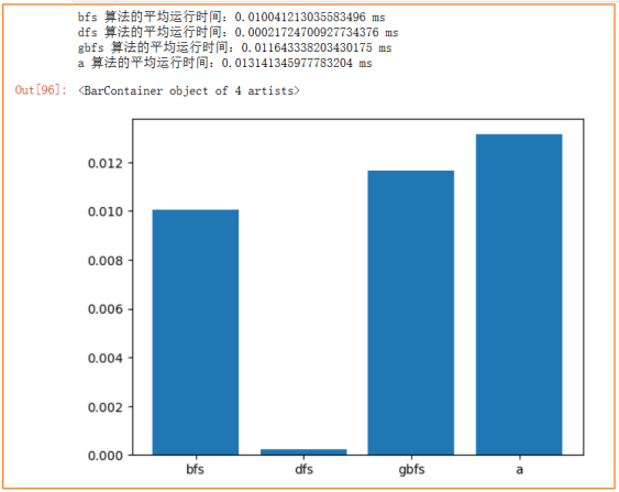
for solve in solve_list:cost_times=[]for i in range(run_n):start_time=time.time()globals()[solve].solve()end_time=time.time()cost_times.append(end_time - start_time)show_time.append(sum(cost_times)*1000/run_n)print(f"{solve} 算法的平均运行时间:{sum(cost_times)*1000/run_n} ms")plt.bar(solve_list,show_time)
将程序运行10000次,统计BFS、DFS、贪婪算法、A*算法的平均运行时间如下:可以看见dfs在问题规模一般的情况的下效率非常高。
扩展思考:设计一个新的启发式函数,并分析该函数的可采纳性和优势(与启发式函数定义为“Zerind到Bucharest的直线距离”相比较)。
假设我们知道每个城市的人口数量,我们可以设计一个启发式函数,该函数将当前节点到目标节点的直线距离与两个城市的人口数量之比作为启发式值。即:fn = 当前节点和目标节点的人口数量之和/目标节点到当前节点的直线距离。
- 可采纳性:这个启发式函数的可采纳性取决于实际问题的特征。如果人口密度对路径规划有重要影响,那么这个启发式函数是可采纳的。例如,人口密度可能会影响交通拥堵程度,从而影响出现体验。
- 优势:与简单的直线距离相比,考虑人口数量可以使得搜索算法更倾向于经过人口稀疏的地区,从而在某些情况下找到更符合实际的路径。例如,如果把油费、乘车体验等等也作为路径选择的依据,那么可以避开人口密集的区域以减少交通拥堵,从而能更快更舒适地到达目的地点。