上一篇Diffusion实战是确确实实一步一步走的公式,这回采用一个更方便的库:diffusers,来实现Diffusion模型训练。
Diffusion实战篇:
【Diffusion实战】训练一个diffusion模型生成S曲线(Pytorch代码详解)
Diffusion综述篇:
【Diffusion综述】医学图像分析中的扩散模型(一)
【Diffusion综述】医学图像分析中的扩散模型(二)
0、所需安装
pip install diffusers  # diffusers库
pip install datasets
1、数据集下载
下载地址:蝴蝶数据集
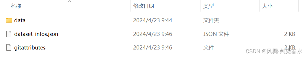
下载好后的文件夹中包括以下文件,放在当前目录下就可以了。
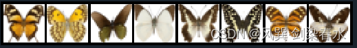
加载数据集,并对一批数据进行可视化:
import torch
import torchvision
from datasets import load_dataset
from torchvision import transforms
import numpy as np
import torch.nn.functional as F
from matplotlib import pyplot as plt
from PIL import Imagedef show_images(x):"""Given a batch of images x, make a grid and convert to PIL"""x = x * 0.5 + 0.5 # Map from (-1, 1) back to (0, 1)grid = torchvision.utils.make_grid(x)grid_im = grid.detach().cpu().permute(1, 2, 0).clip(0, 1) * 255grid_im = Image.fromarray(np.array(grid_im).astype(np.uint8))return grid_imdef transform(examples):images = [preprocess(image.convert("RGB")) for image in examples["image"]]return {"images": images}device = torch.device("cuda" if torch.cuda.is_available() else "cpu")
print(device)# 数据加载
dataset = load_dataset("./smithsonian_butterflies_subset", split='train')image_size = 32
batch_size = 64# 数据增强
preprocess = transforms.Compose([transforms.Resize((image_size, image_size)), # Resizetransforms.RandomHorizontalFlip(), # Randomly flip (data augmentation)transforms.ToTensor(), # Convert to tensor (0, 1)transforms.Normalize([0.5], [0.5]), # Map to (-1, 1)]
)dataset.set_transform(transform)# 数据装载
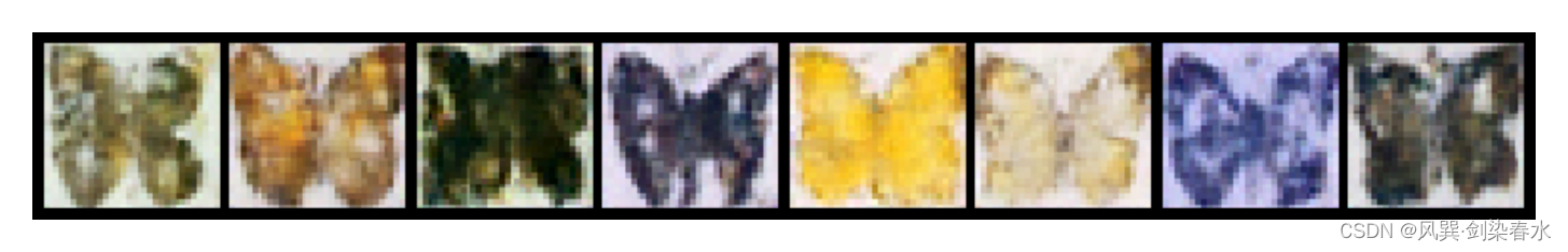
train_dataloader = torch.utils.data.DataLoader(dataset, batch_size=batch_size, shuffle=True)# 抽取一批数据可视化
xb = next(iter(train_dataloader))["images"].to(device)[:8]
print("X shape:", xb.shape)
show_images(xb).resize((8 * 64, 64), resample=Image.NEAREST)
输出可视化结果:
2、加噪调度器
即DDPM论文中需要预定义的 β t {\beta_t } βt ,可使用DDPMScheduler类来定义,其中num_train_timesteps参数为时间步 t {t} t 。
from diffusers import DDPMScheduler# βt值
noise_scheduler = DDPMScheduler(num_train_timesteps=1000)plt.figure(dpi=300)
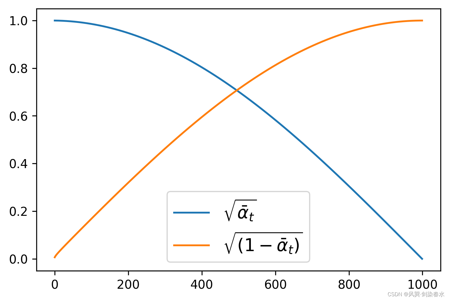
plt.plot(noise_scheduler.alphas_cumprod.cpu() ** 0.5, label=r"${\sqrt{\bar{\alpha}_t}}$")
plt.plot((1 - noise_scheduler.alphas_cumprod.cpu()) ** 0.5, label=r"$\sqrt{(1 - \bar{\alpha}_t)}$")
plt.legend(fontsize="x-large");
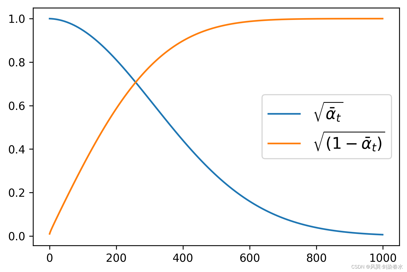
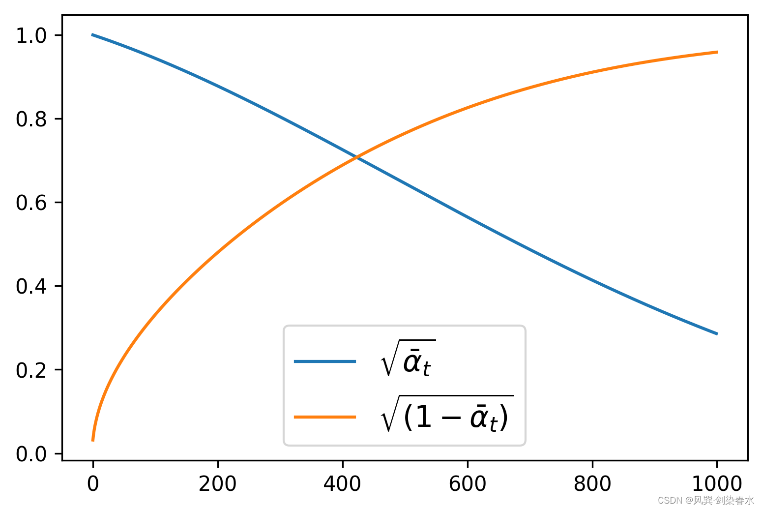
根据定义的 β t {\beta_t } βt ,可视化 α ˉ t {\sqrt {{{\bar \alpha }_t}}} αˉt 和 1 − α ˉ t {\sqrt {1 - {{\bar \alpha }_t}}} 1−αˉt:
通过设置beta_start、beta_end和beta_schedule三个参数来控制噪声调度器的超参数 β t {\beta_t } βt。
noise_scheduler = DDPMScheduler(num_train_timesteps=1000, beta_start=0.001, beta_end=0.004)
beta_schedule可以通过一个函数映射来为模型推理的每一步生成一个 β t {\beta_t } βt值。
noise_scheduler = DDPMScheduler(num_train_timesteps=1000, beta_schedule='squaredcos_cap_v2')
x t = α ˉ t x 0 + 1 − α ˉ t ε {{x_t} = \sqrt {{{\bar \alpha }_t}} {x_0} + \sqrt {1 - {{\bar \alpha }_t}} \varepsilon } xt=αˉtx0+1−αˉtε 加噪前向过程可视化:
timesteps = torch.linspace(0, 999, 8).long().to(device)  # 随机采样时间步
noise = torch.randn_like(xb)
noisy_xb = noise_scheduler.add_noise(xb, noise, timesteps)  # 加噪
print("Noisy X shape", noisy_xb.shape)
show_images(noisy_xb).resize((8 * 64, 64), resample=Image.NEAREST)
输出为:

3、扩散模型定义
diffusers库中模型的定义也非常简洁:
# 创建模型
from diffusers import UNet2DModelmodel = UNet2DModel(sample_size=image_size,  # the target image resolutionin_channels=3,  # the number of input channels, 3 for RGB imagesout_channels=3,  # the number of output channelslayers_per_block=2,  # how many ResNet layers to use per UNet blockblock_out_channels=(64, 128, 128, 256),  # More channels -> more parametersdown_block_types=("DownBlock2D",  # a regular ResNet downsampling block"DownBlock2D","AttnDownBlock2D",  # a ResNet downsampling block with spatial self-attention"AttnDownBlock2D",),up_block_types=("AttnUpBlock2D","AttnUpBlock2D",  # a ResNet upsampling block with spatial self-attention"UpBlock2D","UpBlock2D",  # a regular ResNet upsampling block),
)model.to(device)
with torch.no_grad():model_prediction = model(noisy_xb, timesteps).sample
model_prediction.shape  # 验证输出与输出尺寸相同
4、扩散模型训练
定义优化器,和传统模型一样的训练写法:
# 定义噪声调度器
noise_scheduler = DDPMScheduler(num_train_timesteps=1000, beta_schedule="squaredcos_cap_v2"
)# 优化器
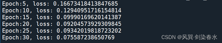
optimizer = torch.optim.AdamW(model.parameters(), lr=4e-4)losses = []for epoch in range(30):for step, batch in enumerate(train_dataloader):clean_images = batch["images"].to(device)# 为图像添加随机噪声noise = torch.randn(clean_images.shape).to(clean_images.device) # epsbs = clean_images.shape[0]# 为每一张图像随机选择一个时间步timesteps = torch.randint(0, noise_scheduler.num_train_timesteps, (bs,), device=clean_images.device).long() # 根据时间步,向清晰的图像中加噪声, 前向过程:根号下αt^ * x0 + 根号下(1-αt^) * epsnoisy_images = noise_scheduler.add_noise(clean_images, noise, timesteps)# 获得模型预测结果noise_pred = model(noisy_images, timesteps, return_dict=False)[0]# 计算损失, 损失回传loss = F.mse_loss(noise_pred, noise) loss.backward(loss)losses.append(loss.item())# 更新模型参数optimizer.step()optimizer.zero_grad()if (epoch + 1) % 5 == 0:loss_last_epoch = sum(losses[-len(train_dataloader) :]) / len(train_dataloader)print(f"Epoch:{epoch+1}, loss: {loss_last_epoch}")
30个epoch训练过程如下所示:
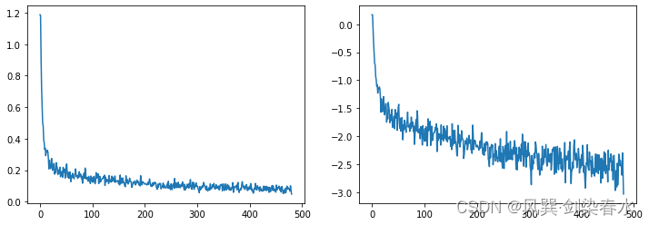
可用以下代码查看损失曲线:
# 损失曲线可视化
fig, axs = plt.subplots(1, 2, figsize=(12, 4))
axs[0].plot(losses)
axs[1].plot(np.log(losses))  # 对数坐标
plt.show()
损失曲线可视化:
5、图像生成
(1)通过建立pipeline生成图像:
# 图像生成
# 方法一:建立一个pipeline, 打包模型和噪声调度器
from diffusers import DDPMPipeline
image_pipe = DDPMPipeline(unet=model, scheduler=noise_scheduler)pipeline_output = image_pipe()
plt.figure()
plt.imshow(pipeline_output.images[0])
plt.axis('off')
plt.show()# 保存pipeline
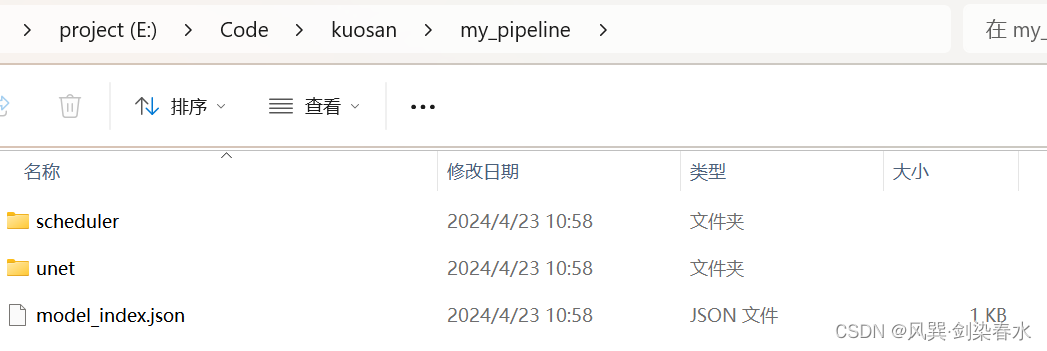
image_pipe.save_pretrained("my_pipeline") # 在当前目录下保存了一个 my_pipeline 的文件夹
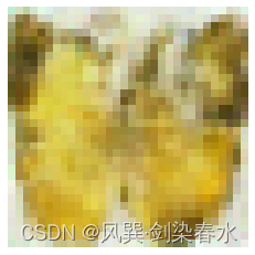
生成的蝴蝶图像如下:
生成的my_pipeline文件夹如下:
(2)通过随机采样循环生成图像:
# 方法二:模型调用, 写采样循环
# 随机初始化8张图像:
sample = torch.randn(8, 3, 32, 32).to(device)for i, t in enumerate(noise_scheduler.timesteps):# 获得模型预测结果with torch.no_grad():residual = model(sample, t).sample# 根据预测结果更新图像sample = noise_scheduler.step(residual, t, sample).prev_sampleshow_images(sample)
8张生成图像如下:
6、代码汇总
import torch
import torchvision
from datasets import load_dataset
from torchvision import transforms
import numpy as np
import torch.nn.functional as F
from matplotlib import pyplot as plt
from PIL import Imagedef show_images(x):"""Given a batch of images x, make a grid and convert to PIL"""x = x * 0.5 + 0.5  # Map from (-1, 1) back to (0, 1)grid = torchvision.utils.make_grid(x)grid_im = grid.detach().cpu().permute(1, 2, 0).clip(0, 1) * 255grid_im = Image.fromarray(np.array(grid_im).astype(np.uint8))return grid_imdef transform(examples):images = [preprocess(image.convert("RGB")) for image in examples["image"]]return {"images": images}# --------------------------------------------------------------------------------
# 1、数据集加载与可视化
device = torch.device("cuda" if torch.cuda.is_available() else "cpu")
print(device)# 数据加载
dataset = load_dataset("./smithsonian_butterflies_subset", split='train')image_size = 32
batch_size = 64# 数据增强
preprocess = transforms.Compose([transforms.Resize((image_size, image_size)),  # Resizetransforms.RandomHorizontalFlip(),  # Randomly flip (data augmentation)transforms.ToTensor(),  # Convert to tensor (0, 1)transforms.Normalize([0.5], [0.5]),  # Map to (-1, 1)]
)dataset.set_transform(transform)# 数据装载
train_dataloader = torch.utils.data.DataLoader(dataset, batch_size=batch_size, shuffle=True)
# --------------------------------------------------------------------------------# --------------------------------------------------------------------------------
# 抽取一批数据可视化
xb = next(iter(train_dataloader))["images"].to(device)[:8]
print("X shape:", xb.shape)
show_images(xb).resize((8 * 64, 64), resample=Image.NEAREST)
# --------------------------------------------------------------------------------# --------------------------------------------------------------------------------
# 2、噪声调度器
from diffusers import DDPMScheduler# 加噪声的系数βt
# noise_scheduler = DDPMScheduler(num_train_timesteps=1000)
# noise_scheduler = DDPMScheduler(num_train_timesteps=1000, beta_start=0.001, beta_end=0.004)
noise_scheduler = DDPMScheduler(num_train_timesteps=1000, beta_schedule='squaredcos_cap_v2')plt.figure(dpi=300)
plt.plot(noise_scheduler.alphas_cumprod.cpu() ** 0.5, label=r"${\sqrt{\bar{\alpha}_t}}$")
plt.plot((1 - noise_scheduler.alphas_cumprod.cpu()) ** 0.5, label=r"$\sqrt{(1 - \bar{\alpha}_t)}$")
plt.legend(fontsize="x-large");
# --------------------------------------------------------------------------------# --------------------------------------------------------------------------------
# 加噪声可视化
timesteps = torch.linspace(0, 999, 8).long().to(device)  # 随机采样时间步
noise = torch.randn_like(xb)
noisy_xb = noise_scheduler.add_noise(xb, noise, timesteps)  # 加噪
print("Noisy X shape", noisy_xb.shape)
show_images(noisy_xb).resize((8 * 64, 64), resample=Image.NEAREST)
# --------------------------------------------------------------------------------# --------------------------------------------------------------------------------
# 3、创建模型
from diffusers import UNet2DModelmodel = UNet2DModel(sample_size=image_size,  # the target image resolutionin_channels=3,  # the number of input channels, 3 for RGB imagesout_channels=3,  # the number of output channelslayers_per_block=2,  # how many ResNet layers to use per UNet blockblock_out_channels=(64, 128, 128, 256),  # More channels -> more parametersdown_block_types=("DownBlock2D",  # a regular ResNet downsampling block"DownBlock2D","AttnDownBlock2D",  # a ResNet downsampling block with spatial self-attention"AttnDownBlock2D",),up_block_types=("AttnUpBlock2D","AttnUpBlock2D",  # a ResNet upsampling block with spatial self-attention"UpBlock2D","UpBlock2D",  # a regular ResNet upsampling block),
)model.to(device)
with torch.no_grad():model_prediction = model(noisy_xb, timesteps).sample
model_prediction.shape  # 验证输出与输出尺寸相同
# --------------------------------------------------------------------------------# --------------------------------------------------------------------------------
# 4、扩散模型训练
# 定义噪声调度器
noise_scheduler = DDPMScheduler(num_train_timesteps=1000, beta_schedule="squaredcos_cap_v2"
)# 优化器
optimizer = torch.optim.AdamW(model.parameters(), lr=4e-4)losses = []for epoch in range(30):for step, batch in enumerate(train_dataloader):clean_images = batch["images"].to(device)# 为图像添加随机噪声noise = torch.randn(clean_images.shape).to(clean_images.device)  # epsbs = clean_images.shape[0]# 为每一张图像随机选择一个时间步timesteps = torch.randint(0, noise_scheduler.num_train_timesteps, (bs,), device=clean_images.device).long()  # 根据时间步,向清晰的图像中加噪声, 前向过程:根号下αt^ * x0 + 根号下(1-αt^) * epsnoisy_images = noise_scheduler.add_noise(clean_images, noise, timesteps)# 获得模型预测结果noise_pred = model(noisy_images, timesteps, return_dict=False)[0]# 计算损失, 损失回传loss = F.mse_loss(noise_pred, noise)  loss.backward(loss)losses.append(loss.item())# 更新模型参数optimizer.step()optimizer.zero_grad()if (epoch + 1) % 5 == 0:loss_last_epoch = sum(losses[-len(train_dataloader) :]) / len(train_dataloader)print(f"Epoch:{epoch+1}, loss: {loss_last_epoch}")
# --------------------------------------------------------------------------------# --------------------------------------------------------------------------------
# 损失曲线可视化
fig, axs = plt.subplots(1, 2, figsize=(12, 4))
axs[0].plot(losses)
axs[1].plot(np.log(losses))  # 对数坐标
plt.show()
# --------------------------------------------------------------------------------# --------------------------------------------------------------------------------
# 5、图像生成
# 方法一:建立一个pipeline, 打包模型和噪声调度器
from diffusers import DDPMPipeline
image_pipe = DDPMPipeline(unet=model, scheduler=noise_scheduler)pipeline_output = image_pipe()plt.figure()
plt.imshow(pipeline_output.images[0])
plt.axis('off')
plt.show()image_pipe.save_pretrained("my_pipeline")  # 在当前目录下保存了一个 my_pipeline 的文件夹# 方法二:模型调用, 写采样循环
# 随机初始化8张图像:
sample = torch.randn(8, 3, 32, 32).to(device)for i, t in enumerate(noise_scheduler.timesteps):# 获得模型预测结果with torch.no_grad():residual = model(sample, t).sample# 根据预测结果更新图像sample = noise_scheduler.step(residual, t, sample).prev_sampleshow_images(sample)grid_im = show_images(sample).resize((8 * 64, 64), resample=Image.NEAREST)
plt.figure(dpi=300)
plt.imshow(grid_im)
plt.axis('off')
plt.show()
# --------------------------------------------------------------------------------
参考资料:扩散模型从原理到实践. 人民邮电出版社. 李忻玮, 苏步升等.
diffusers确实很方便使用,有点子PyCaret的感觉了~