参考与前言
此教程首次书写于2021年12月份 至 2022年4月份间不断补充;阅读本文时可以对着代码运行查看
- 官方网址:https://pytorch.org/tutorials/ 【基本从这里翻译而来 更简洁版+碎碎念】
- https://pytorch.org/tutorials/beginner/blitz/cifar10_tutorial.html#sphx-glr-beginner-blitz-cifar10-tutorial-py
- 简单版分类器:https://pytorch.org/tutorials/beginner/blitz/cifar10_tutorial.html
好像还是很tensorflow有点区别的 毕竟 tensorflow emmm 我看一下 好像懂了,我记得久远之前我看过pytorch的 但是因为没做笔记+好久没用了 所以 忘得也挺快
相关训练细节上加速的tutorial:Tutorial: GPU利用率问题 [V]
1. 数据结构
tensor
tensor 是一种特殊的数据结构,与数组和矩阵非常相似。在 PyTorch 中,我们使用 tensor 对模型的输入和输出以及模型的参数进行编码。
-
好吧 torch.from_numpy 也很快 emm
初始化方法
# Directly from data
data = [[1, 2], [3, 4]]
x_data = torch.tensor(data)# From a NumPy array
np_array = np.array(data)
x_np = torch.from_numpy(np_array)# From another tensor:
x_ones = torch.ones_like(x_data) # retains the properties of x_data
print(f"Ones Tensor: \n {x_ones} \n")
x_rand = torch.rand_like(x_data, dtype=torch.float) # overrides the datatype of x_data
print(f"Random Tensor: \n {x_rand} \n")# With random or constant values:
shape = (2, 3,)
rand_tensor = torch.rand(shape)
ones_tensor = torch.ones(shape)
zeros_tensor = torch.zeros(shape)print(f"Random Tensor: \n {rand_tensor} \n")
print(f"Ones Tensor: \n {ones_tensor} \n")
print(f"Zeros Tensor: \n {zeros_tensor}")
可以 from numpy 当然也可以to numpy啦,Changes in the NumPy array reflects in the tensor.
t = torch.ones(5)
print(f"t: {t}")
n = t.numpy()
print(f"n: {n}")t.add_(1)
print(f"t: {t}")
print(f"n: {n}")t: tensor([2., 2., 2., 2., 2.])
n: [2. 2. 2. 2. 2.]
Attribute
就是类似numpy里面的.shape, type(), 以及其特有的存储地点:描述它们的形状、数据类型和存储它们的设备。
tensor = torch.rand(3, 4)print(f"Shape of tensor: {tensor.shape}")
print(f"Datatype of tensor: {tensor.dtype}")
print(f"Device tensor is stored on: {tensor.device}")
操作
换个地方放放:
# We move our tensor to the GPU if available
if torch.cuda.is_available():tensor = tensor.to('cuda')print(f"Device tensor is stored on: {tensor.device}")# 和numpy基本一模一样的操作形式
tensor = torch.ones(4, 4)
tensor[:,1] = 0
print(tensor)tensor([[1., 0., 1., 1.],[1., 0., 1., 1.],[1., 0., 1., 1.],[1., 0., 1., 1.]])# -------------------------------------------------
# 把几个tensor合在一起
t1 = torch.cat([tensor, tensor, tensor], dim=1)
print(t1)tensor([[1., 0., 1., 1., 1., 0., 1., 1., 1., 0., 1., 1.],[1., 0., 1., 1., 1., 0., 1., 1., 1., 0., 1., 1.],[1., 0., 1., 1., 1., 0., 1., 1., 1., 0., 1., 1.],[1., 0., 1., 1., 1., 0., 1., 1., 1., 0., 1., 1.]])# -------------------------------------------------# 对应位置的元素相乘
# This computes the element-wise product
print(f"tensor.mul(tensor) \n {tensor.mul(tensor)} \n")
# Alternative syntax:
print(f"tensor * tensor \n {tensor * tensor}")# 矩阵的形式
# This computes the matrix multiplication between two tensors
print(f"tensor.matmul(tensor.T) \n {tensor.matmul(tensor.T)} \n")
# Alternative syntax:
print(f"tensor @ tensor.T \n {tensor @ tensor.T}")# -------------------------------------------------
print(tensor, "\n")
tensor.add_(5)
print(tensor)tensor([[1., 0., 1., 1.],[1., 0., 1., 1.],[1., 0., 1., 1.],[1., 0., 1., 1.]])tensor([[6., 5., 6., 6.],[6., 5., 6., 6.],[6., 5., 6., 6.],[6., 5., 6., 6.]])
In-place operations Operations that have a _ suffix are in-place. For example: x.copy_(y), x.t_(), will change x.
2. 数据与加载
处理数据样本的代码可能会变得混乱且难以维护; 我们希望数据集代码与模型训练代码分离,以获得更好的可读性和模块化。pytorch提供了两个数据的使用库: torch.utils.data.DataLoader and torch.utils.data.Dataset that allow you to use pre-loaded datasets as well as your own data.
Datasetstores the samples and their corresponding labelsDataLoaderwraps an iterable around theDatasetto enable easy access to the samples.
当然pytorch里的Dataset 也有一些开源的数据集成,更多查询: Image Datasets, Text Datasets, and Audio Datasets
FashionMNIST
import torch
from torch.utils.data import Dataset
from torchvision import datasets
from torchvision.transforms import ToTensor
import matplotlib.pyplot as plttraining_data = datasets.FashionMNIST(root="data",train=True,download=True,transform=ToTensor()
)test_data = datasets.FashionMNIST(root="data",train=False,download=True,transform=ToTensor()
)labels_map = {0: "T-Shirt",1: "Trouser",2: "Pullover",3: "Dress",4: "Coat",5: "Sandal",6: "Shirt",7: "Sneaker",8: "Bag",9: "Ankle Boot",
}
figure = plt.figure(figsize=(8, 8))
cols, rows = 3, 3
for i in range(1, cols * rows + 1):sample_idx = torch.randint(len(training_data), size=(1,)).item()img, label = training_data[sample_idx]figure.add_subplot(rows, cols, i)plt.title(labels_map[label])plt.axis("off")plt.imshow(img.squeeze(), cmap="gray")
plt.show()

Custom Dataset
自定义的Dataset必须有这三个函数: init, len, and getitem.
对应 FashionMNIST 的数据集,其照片是存在 img_dir文件夹中 and their labels are stored separately in a CSV file annotations_file.
官方示例:
import os
import pandas as pd
from torchvision.io import read_imageclass CustomImageDataset(Dataset):def __init__(self, annotations_file, img_dir, transform=None, target_transform=None):self.img_labels = pd.read_csv(annotations_file)self.img_dir = img_dirself.transform = transformself.target_transform = target_transformdef __len__(self):return len(self.img_labels)def __getitem__(self, idx):img_path = os.path.join(self.img_dir, self.img_labels.iloc[idx, 0])image = read_image(img_path)label = self.img_labels.iloc[idx, 1]if self.transform:image = self.transform(image)if self.target_transform:label = self.target_transform(label)return image, label
init
init 函数仅在你实例化这个Dataset object的时候运行一次. 我们在这里给出包含图片,label和是否需要转换
如果一个labels.csv文件长这样的话:
tshirt1.jpg, 0
tshirt2.jpg, 0
......
ankleboot999.jpg, 9
那么__init__函数为:
def __init__(self, annotations_file, img_dir, transform=None, target_transform=None):self.img_labels = pd.read_csv(annotations_file, names=['file_name', 'label'])self.img_dir = img_dirself.transform = transformself.target_transform = target_transform
len
这个函数主要返回我们数据集的大小,比如:
def __len__(self):return len(self.img_labels)
getitem
这个函数主要用来加载输入的 idx 对应的数据,基于给的idx,可以定位到哪张图片,然后使用 read_image 转成tensor,从 self.img_labels找到对应的label,然后返回tensor格式的图片和一个tuple格式的label
def __getitem__(self, idx):img_path = os.path.join(self.img_dir, self.img_labels.iloc[idx, 0])image = read_image(img_path)label = self.img_labels.iloc[idx, 1]if self.transform:image = self.transform(image)if self.target_transform:label = self.target_transform(label)return image, label
transforms
数据并不总是以训练机器学习算法所需的最终处理形式出现。 我们使用转换来对数据进行一些操作并使其适合训练。
从上一条我们知道需要返回tensor格式的数据,如image可能直接可以从库里调用ToTensor()
TorchVision 库里的数据集,通常有两个参数
transformto modify the featurestarget_transformto modify the labels - that accept callables containing the transformation logic.
torchvision.transforms 这个模块,已经提供了很多通用的transform的功能
例如以下,同样FashionMNIST 这个数据集下 feature图片是PIL图片格式,label是整数;为了训练,我们需要把feature归一化成tensors,把label用one-hot encoded的tensor表示,为了实现这些呢:我们就需要使用 ToTensor and Lambda. 比如这里:比前面的多了一行对label的转换
import torch
from torchvision import datasets
from torchvision.transforms import ToTensor, Lambdads = datasets.FashionMNIST(root="data",train=True,download=True,transform=ToTensor(),target_transform=Lambda(lambda y: torch.zeros(10, dtype=torch.float).scatter_(0, torch.tensor(y), value=1))
)
比如最近参加kaggle竞赛练手的,写了关于image的transforms
preprocess = transforms.Compose([transforms.Resize(256),transforms.CenterCrop(224),transforms.ToTensor(),transforms.Normalize(mean=[0.485, 0.456, 0.406], std=[0.229, 0.224, 0.225]),
])
ToTensor()
ToTensor 是把PIL图片或者是numpy的ndarray转成 FloatTensor. 然后图片的像素intensity值都归一化到[0., 1.]
Lambda Transforms
Lambda 转换适用于任何用户定义的 lambda 函数。 在这里,我们定义了一个函数来将整数转换为单one-hot tensor。 它首先创建一个大小为 10(我们数据集中的标签数量)的zero tensor,并调用 scatter_,它在标签 y 给定的索引上分配一个值=1
target_transform = Lambda(lambda y: torch.zeros(10, dtype=torch.float).scatter_(dim=0, index=torch.tensor(y), value=1))
3. 网络NetWork
构建网络
神经网络由对数据执行操作的层/模块组成。 torch.nn 命名空间提供了构建自己的神经网络所需的所有构建块。 PyTorch 中的每个模块都是 nn.Module 的子类。 神经网络是一个模块,由其他模块(层)组成。 这种嵌套结构允许轻松构建和管理复杂的架构。
在下面是构建一个神经网络来对 FashionMNIST 数据集中的图像进行分类的一个例子
import os
import torch
from torch import nn
from torch.utils.data import DataLoader
from torchvision import datasets, transformsdevice = 'cuda' if torch.cuda.is_available() else 'cpu'
print(f'Using {device} device')class NeuralNetwork(nn.Module):def __init__(self):super(NeuralNetwork, self).__init__()self.flatten = nn.Flatten()self.linear_relu_stack = nn.Sequential(nn.Linear(28*28, 512),nn.ReLU(),nn.Linear(512, 512),nn.ReLU(),nn.Linear(512, 10),)def forward(self, x):x = self.flatten(x)logits = self.linear_relu_stack(x)return logitsmodel = NeuralNetwork().to(device)
print(model)
通过继承 nn.Module 来定义我们的神经网络,并在 __init__ 中初始化神经网络层。 每个 nn.Module 子类都在 forward 方法中实现对输入数据的操作。
-
这里就是和tensorflow不太一样的地方,比如这里tensorflow定义完后 直接是 .fit 然后就是trainde 过程了
# Creat a neural network now
model_cnn = Sequential(name = "CNN")# First Convolution Layer
model_cnn.add(Conv2D(8, input_shape = x_trainr.shape[1:], kernel_size = 3,padding='same',strides=1,activation='relu'))
model_cnn.add(MaxPooling2D(pool_size=2))# 2nd Convolution Layer
model_cnn.add(Conv2D(16,kernel_size = 3,padding='same',strides=1,activation='relu'))
model_cnn.add(MaxPooling2D(pool_size=2))# Fully connected layer
model_cnn.add(Flatten())
model_cnn.add(Dense(64))
model_cnn.add(Activation("relu"))# Last Fully connected layer
model_cnn.add(Dense(11))model_cnn.add(Activation("softmax"))
model_cnn.compile(loss = "sparse_categorical_crossentropy",optimizer="adam",metrics=['accuracy'])
model_cnn.summary()
model_cnn.fit(x_trainr,y_train,epochs=10)
print("Test Dataset:")
test_loss, test_acc = model_cnn.evaluate(x_testr,y_test)
使用将data传到模型里就行,它会自动运行 model’s forward, 同时还有 background operations. 不需要自己调用 model.forward() directly!
在输入上调用模型会返回一个 10D tensor,其中包含每个类的原始预测值。 我们通过将其传递给 nn.Softmax 模块的实例来获得预测概率。
X = torch.rand(1, 28, 28, device=device)
logits = model(X)
pred_probab = nn.Softmax(dim=1)(logits)
y_pred = pred_probab.argmax(1)
print(f"Predicted class: {y_pred}")
-
原来是自己写ephoc来训练
block 形式的
参考于:5. 深度学习计算 - 动手学深度学习 2.0.0-beta0 documentation
训练方法
直接快进到这里了,这个是示例里的:
import torch.nn as nn
import torch.nn.functional as F# 1. 导入数据
transform = transforms.Compose([transforms.ToTensor(),transforms.Normalize((0.5, 0.5, 0.5), (0.5, 0.5, 0.5))])
batch_size = 4
trainset = torchvision.datasets.CIFAR10(root='./data', train=True,download=True, transform=transform)
trainloader = torch.utils.data.DataLoader(trainset, batch_size=batch_size,shuffle=True, num_workers=2)
testset = torchvision.datasets.CIFAR10(root='./data', train=False,download=True, transform=transform)
testloader = torch.utils.data.DataLoader(testset, batch_size=batch_size,shuffle=False, num_workers=2)
classes = ('plane', 'car', 'bird', 'cat','deer', 'dog', 'frog', 'horse', 'ship', 'truck')# 2. 定义网络层
class Net(nn.Module):def __init__(self):super().__init__()self.conv1 = nn.Conv2d(3, 6, 5)self.pool = nn.MaxPool2d(2, 2)self.conv2 = nn.Conv2d(6, 16, 5)self.fc1 = nn.Linear(16 * 5 * 5, 120)self.fc2 = nn.Linear(120, 84)self.fc3 = nn.Linear(84, 10)def forward(self, x):x = self.pool(F.relu(self.conv1(x)))x = self.pool(F.relu(self.conv2(x)))x = torch.flatten(x, 1) # flatten all dimensions except batchx = F.relu(self.fc1(x))x = F.relu(self.fc2(x))x = self.fc3(x)return xnet = Net()# 3. 评判器
import torch.optim as optim
criterion = nn.CrossEntropyLoss()
optimizer = optim.SGD(net.parameters(), lr=0.001, momentum=0.9)# 4. 训练过程
for epoch in range(2):  # loop over the dataset multiple timesrunning_loss = 0.0for i, data in enumerate(trainloader, 0):# get the inputs; data is a list of [inputs, labels]inputs, labels = data# zero the parameter gradientsoptimizer.zero_grad()# forward + backward + optimizeoutputs = net(inputs)loss = criterion(outputs, labels)loss.backward()optimizer.step()# print statisticsrunning_loss += loss.item()if i % 2000 == 1999:    # print every 2000 mini-batchesprint('[%d, %5d] loss: %.3f' % (epoch + 1, i + 1, running_loss / 2000))running_loss = 0.0
print('Finished Training')# 5. save model
PATH = './cifar_net.pth'
torch.save(net.state_dict(), PATH)# 6. 从测试集中弄一些出来
dataiter = iter(testloader)
images, labels = dataiter.next()# print images
imshow(torchvision.utils.make_grid(images))
print('GroundTruth: ', ' '.join('%5s' % classes[labels[j]] for j in range(4)))# 7. 打开原来的model
net = Net()
net.load_state_dict(torch.load(PATH))# 8. 输出output
outputs = net(images)
_, predicted = torch.max(outputs, 1)
print('Predicted: ', ' '.join('%5s' % classes[predicted[j]]for j in range(4)))
动态调整 learning rate
参考,此处需要注意文档的版本选择,因为1.10后的torch实现了更多动态调整的方式:torch.optim - PyTorch 1.10.1 documentation
使用方式参考:
import torch.optim as optim
net = MODEL(out_label = len(classes)).to(device)criterion = nn.CrossEntropyLoss()
optimizer = optim.SGD(net.parameters(), lr=lr)# 动态改变Learning rate
scheduler = optim.lr_scheduler.StepLR(optimizer, step_size=5, gamma=0.5)# 4. 训练过程
for epoch in tqdm(range(num_epochs)):  # loop over the dataset multiple timesfor i, data in enumerate(train_dataloader,0):# get the inputs; data is a list of [inputs, labels]inputs, labels = datainputs, labels = inputs.to(device), labels.to(device)# zero the parameter gradientsoptimizer.zero_grad()# forward + backward + optimizeoutputs = net(inputs)loss = criterion(outputs, labels)loss.backward()optimizer.step()scheduler.step()
4. 数据操作
由杰哥代码发现的一个更好用的:rearrange
rearrange - Einops
Pytorch view() permute() contiguous() transpose()
view
CSDN介绍;官网介绍
import torch
from torch import nn
from torch.utils.data import DataLoader
from torchvision import datasets
from torchvision.transforms import ToTensor, Lambda, Compose
import matplotlib.pyplot as pltx = torch.rand(24,3,256,256)
x.size()a = x.view(x.size(0), -1)
print('after view',a.size())m = nn.Sequential(nn.Flatten())
y = m(x)
print('after flatten',y.size())
有意思的是,CSDN 下有人问了 和flatten有什么区别 这个操作,从数据输出上来看,都是一样的输出 [24,196608] ,而且展开的数据也都是一样的,关于这个我提了一个问 有人回答了 真不错呀,省流版:一般大家在model中都会习惯性nn.Flatten()
YP大哥:好像是某个开的空间是连续的
-
但是我实践了一下 并没有什么区别?首先是关于contiguous说的是返回和原数据一样的形式的连续空间tensor,但是我一改b/y 还是会对其他造成影响,也就是说明 =和=.contiguous 都是直接指向了原tensor的地址?→ 但这点我实际vscode debug的时候发现地址并不一样

December 14, 2021 10:22 PM (GMT+8) 刚刚又仔细看了一下,是这样的view的操作需要这个tensor在连续的空间呢,所以呢一般都会在view操作前先contiguous,使其放在一个连续的内存空间上
contiguous
将数据放在连续空间内存下,一般在view操作前会用一下,因为tensor经过permute,
permute
torch官方
torch.permute(input, dims) → Tensor
- input (Tensor) – 输出的tensor数据
- dims (tuple of python:ints) – 想要的维度的顺序
举个例子,在这里 2,0,1 表示 我希望第二个维度(也就是size 5那里)在第0个,第零个维度在第1个,第一个维度在第2个【以0为开始哈】
x = torch.randn(2, 3, 5)
x.size()
torch.permute(x, (2, 0, 1)).size()
所以permute后,size就变成了(5,2,3)
sqeeze 和 unsqeeze
- torch.squeeze():这个函数主要对数据的维度进行压缩,去掉维数为1的的维度,默认是将a中所有为1的维度删掉。也可以通过dim指定位置,删掉指定位置的维数为1的维度。
- torch.unsqueeze():这个函数主要是对数据维度进行扩充。需要通过dim指定位置,给指定位置加上维数为1的维度。
这里是关于squeeze和unsqueeze的图示 (图片摘自stackexchange):

赠人点赞 手有余香 😆;正向回馈 才能更好开放记录 hhh