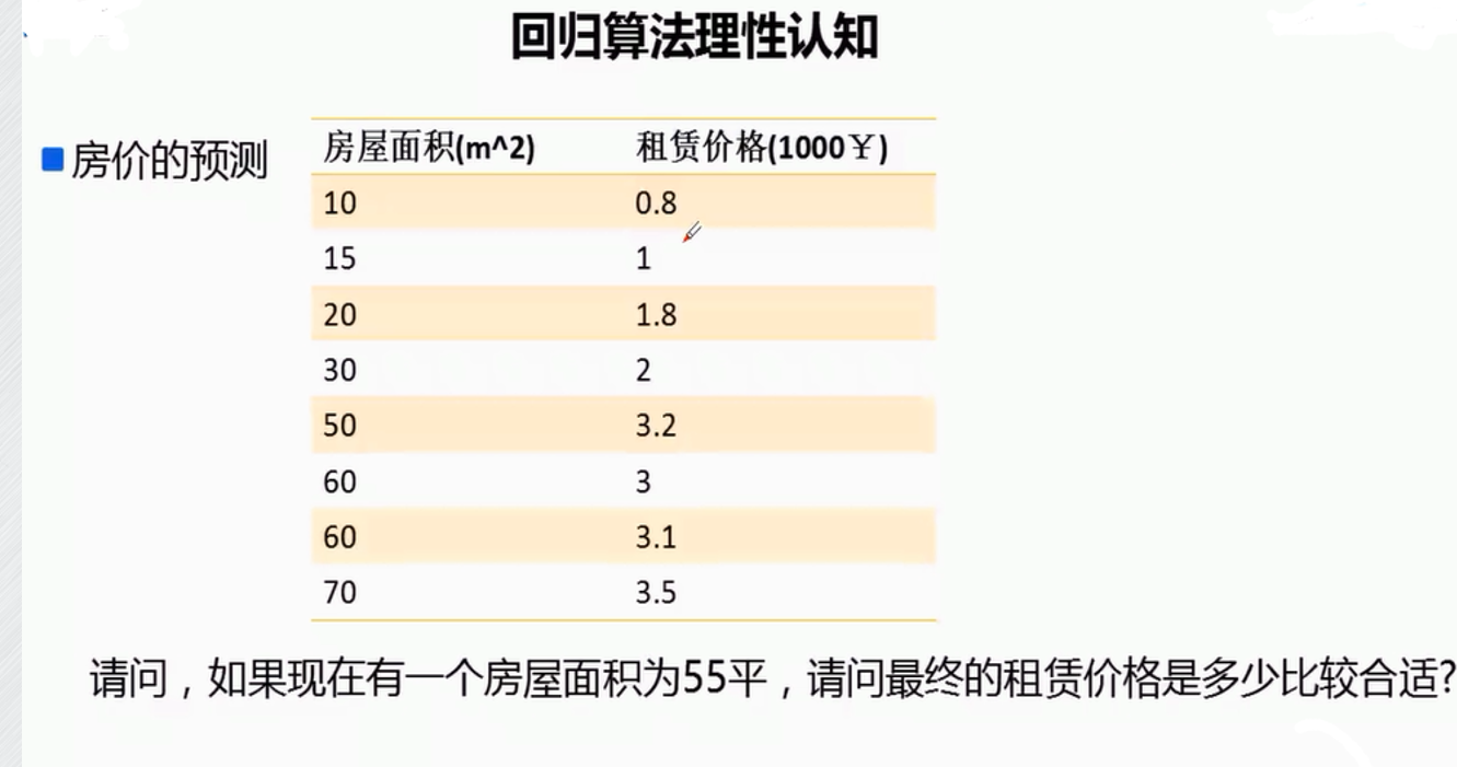
线性回归
一元:
(1)手工最小二乘法
import numpy as np
a=np.loadtxt("homespace_price",delimiter=',',dtype=float)
homespace=a[:,0]
price=a[:,1]
x_avg=np.average(homespace)
y_avg=np.average(price)
xfang_avg=np.average(homespace*homespace)
xy_avg=np.average(homespace*price)
w=(xy_avg-x_avg*y_avg)/(xfang_avg-(x_avg*x_avg))
b=y_avg-w*x_avg
price_predict=w*55+b
print("预测55平方米的房子价格:%f" %price_predict)
(2)sklearn自带的LinearRegression
from sklearn.linear_model import LinearRegression as LR
import sklearn.preprocessing as pr
import numpy as np
a=np.loadtxt("data",delimiter=',',dtype=float)
X=a[:,0].reshape(-1,1)
Y=a[:,1].reshape(-1,1)
scaler=pr.StandardScaler()
scaler.fit(X)
#归一化自变量
x_train=scaler.transform(X)
x_test=scaler.transform(np.array([55]).reshape(1,-1))
modle=LR()
modle.fit(x_train,Y)
print(modle.predict(x_test))
print(modle.coef_) # Coefficient of the features 决策函数中的特征系数
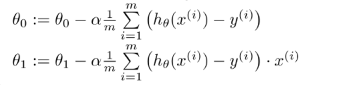
print(modle.intercept_) # 又名bias偏置,若设置为False,则为0(3)梯度下降算法
1/m是个常数可以包括在学习率a中不用单独写
核心公式
不用矩阵
import numpy as np
it=1000#迭代次数
a=0.0001#学习率(步长)
f=np.loadtxt("houseprice",dtype=float,delimiter=',')
x_train=f[:,0:1].reshape(-1,1)
y_train=f[:,1].reshape(-1,1)
num = f.shape[0]
k=1
b=0
#迭代1000次
for i in range(it):td=0for j in range(num):td+=k*x_train[j][0]+b-y_train[j][0]#相当于求和所有差距k=k-(a*td*x_train[j])/numb=b-(a*td)/num
print(k*55+b)
用矩阵
import numpy as np
a=0.0001#学习率
it=1000#迭代次数
f=np.loadtxt("houseprice",delimiter=",",dtype=float)
x_train1=np.concatenate((np.ones((f.shape[0],1)),f[:,0].reshape(-1,1)),axis=1)
y_train1=f[:,1].reshape(-1,1)
w=np.array([0.0,0.0]).reshape(-1,1)
for i in range(it):#迭代td=x_train1.dot(w)-y_train1w=w-a*x_train1.T.dot(td)
x_test1=np.array([1,55]).reshape(1,-1)
print(x_test1.dot(w))
多元:
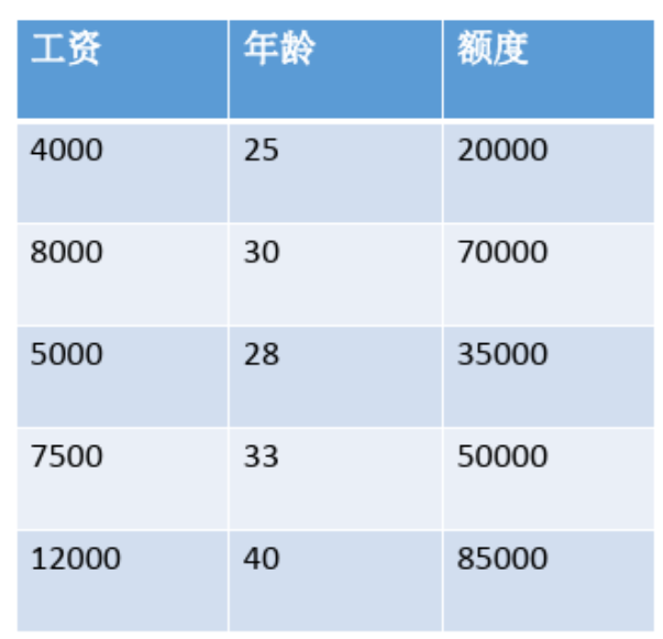
(1)手动最小二乘法
最左边一列补充上全1
import numpy as np
a=np.loadtxt("salaryage",delimiter=',',dtype=int)
X=a[:,0:2].reshape(-1,2)
Y=a[:,2].reshape(-1,1)
X_train=np.concatenate((np.ones((a.shape[0],1)),X),axis=1)#增加一列1以后的训练集
w=np.linalg.inv(X_train.T.dot(X_train)).dot(X_train.T.dot(Y))
X_test=np.array([1,18000,50]).reshape(1,-1)
y_predict=X_test.dot(w)
print(y_predict)
(2)sklearn里面的LinearRegression
import numpy as np
import sklearn.preprocessing as pre
from sklearn.linear_model import LinearRegression
a=np.loadtxt("salaryage1",dtype=int,delimiter=',')
xtrain=a[:,0:2].reshape(-1,2)
ytrain=a[:,2].reshape(-1,1)
scaler=pre.StandardScaler()
# #标准化
scaler.fit(xtrain)
x_test=np.array([18000,50]).reshape(1,-1)
x_test=scaler.transform(x_test)
xtrain=scaler.transform(xtrain)
#线性回归
modle=LinearRegression()
modle.fit(xtrain,ytrain)
print(modle.predict(x_test))
(3)梯度下降算法
关键是因为这里的两个自变量因为量纲不同所以需要先归一化去除单位影响
除此之外这里计算步骤如一元用矩阵那个
import numpy as np# 数据
data = np.array([[4000, 25, 20000],[8000, 30, 70000],[5000, 28, 35000],[7500, 33, 50000],[12000, 40, 85000]
])# 特征和标签
x = data[:, :2]
y = data[:, 2].reshape(-1, 1)# 数据标准化(Z-score标准化)
x_mean = np.mean(x, axis=0)
x_std = np.std(x, axis=0)
x = (x - x_mean) / x_std
print(x)
# 添加一列全为1的列向量,用于截距项
x = np.concatenate((np.ones((x.shape[0], 1)), x), axis=1)# 初始化参数
w = np.zeros((x.shape[1], 1))# 学习率
alpha = 0.001
# 迭代次数
it = 1000# 样本数量
n = x.shape[0]# 梯度下降迭代
for i in range(it):# 计算梯度gradient =   x.T.dot(x.dot(w) - y)# 更新参数w = w - alpha * gradient# 新数据(工资18000,工龄50)
new_data = np.array([18000, 50]).reshape(1, -1)
# 对新数据进行同样的标准化处理
new_data = (new_data - x_mean) / x_std
new_data = np.concatenate((np.ones((new_data.shape[0], 1)), new_data), axis=1)# 预测
prediction = new_data.dot(w)
print("预测的贷款额度为:", prediction[0][0])