YOLOv5-6.1源码详解之损失函数loss.py-编程知识

1 目标检测结果精确度的度量

2 YOLOv5-6.1损失函数

2.1 classification类别损失

2.2 confidence置信度损失

2.3 localization定位损失

3 YOLOv5-6.1损失函数loss.py代码解析

3.1 class ComputeLoss

3.1.1 __init__

3.1.2 build_targets

3.1.3 _call__

3.2 smooth_BCE

3.3 BCEBlurWithLogitsLoss

3.4 FocalLoss

References

1 目标检测结果精确度的度量

目标检测任务有三个主要目的：

检测出图像中目标的位置，同一张图像中可能存在多个检测目标；
检测出目标的大小，通常为恰好包围目标的矩形框；
对检测到的目标进行识别分类。

所以，判断检测结果精确不精确，主要基于以上三个目的来衡量：

首先我们来定义理想情况：图像中实际存在目标的所有位置，都被检测出来。检测结果越接近这个理想状态，也即漏检/误检的目标越少，则认为结果越精确；
同样定义理想情况：检测到的矩形框恰好能包围检测目标。检测结果越接近这个理想状态，那么认为结果越精确；
对检测到的目标，进行识别与分类，分类结果与目标的实际分类越符合，说明结果越精确。

如下图所示，人、大巴为检测目标，既要检测出所有人和大巴的位置，也要检测出包围人和大巴的最小矩形框，同时还要识别出哪个矩形框内是人，哪个矩形框内是大巴。

2 YOLOv5-6.1损失函数

通过阅读YOLOv5-6.1版本中的loss.py文件可知，YOLOv5的损失函数包括：

classification loss 分类损失
localization loss 定位损失，预测框和真实框之间的误差
confidence loss 置信度损失，框的目标性

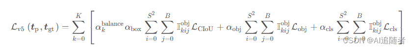
三个部分的损失均是通过匹配到的正样本对来计算，每一个输出特征图相互独立，直接相加得到最终每一部分的损失值。先给出整体的计算公式：

2.1 classification类别损失

类别损失与置信度损失类似，通过预测框的类别分数和目标框类别的one-hot表现来计算类别损失，公式如下：

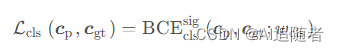
这里目标置信度损失和类别损失使用的是带 sigmoid 的二进制交叉熵函数 BCEWithLogitsLoss。如果要使用 Focal Loss 在其基础上改动即可。

BCEcls = nn.BCEWithLogitsLoss(pos_weight=torch.tensor([h['cls_pw']], device=device))
lcls += self.BCEcls(pi[..., 5:], t_cls)

2.2 confidence置信度损失

目标置信度损失由正样本匹配得到的样本对计算，一是预测框中的目标置信度分数 $p_{o}$ ；二是预测框和与之对应的目标框的 iou 值，其作为 ground-truth。两者计算二进制交叉熵得到最终的目标置信度损失。公式如下：

BCEobj = nn.BCEWithLogitsLoss(pos_weight=torch.tensor([h['obj_pw']], device=device))
obji = self.BCEobj(pi[..., 4], tobj)

2.3 localization定位损失

YOLOv5使用的是CIoU Loss，具体CIoU Loss分析可以参考优化改进YOLOv5算法之添加GIoU、DIoU、CIoU、EIoU、Wise-IoU模块(超详细)_eiou代码-CSDN博客YOLOv5 中正样本匹配策略和bbox回归如下图所示。

iou_term = bbox_iou(pbox.T, tbox[i], x1y1x2y2=False, CIoU=True)
lbox += (1.0 - iou_term).mean()

3 YOLOv5-6.1损失函数loss.py代码解析

3.1 class ComputeLoss

3.1.1 init

代码和注释如下：

  def __init__(self, model, autobalance=False):super(ComputeLoss, self).__init__()device = next(model.parameters()).device  # get model deviceh = model.hyp  # hyperparameters'''定义分类损失和置信度损失为带sigmoid的二值交叉熵损失，即会先将输入进行sigmoid再计算BinaryCrossEntropyLoss(BCELoss)。pos_weight参数是正样本损失的权重参数。'''# Define criteriaBCEcls = nn.BCEWithLogitsLoss(pos_weight=torch.tensor([h['cls_pw']], device=device))BCEobj = nn.BCEWithLogitsLoss(pos_weight=torch.tensor([h['obj_pw']], device=device))'''对标签做平滑,eps=0就代表不做标签平滑,那么默认cp=1,cn=0后续对正类别赋值cp，负类别赋值cn'''# Class label smoothing https://arxiv.org/pdf/1902.04103.pdf eqn 3self.cp, self.cn = smooth_BCE(eps=h.get('label_smoothing', 0.0))  # positive, negative BCE targets'''超参设置g>0则计算FocalLoss'''# Focal lossg = h['fl_gamma']  # focal loss gammaif g > 0:BCEcls, BCEobj = FocalLoss(BCEcls, g), FocalLoss(BCEobj, g)'''获取detect层'''det = model.module.model[-1] if is_parallel(model) else model.model[-1]  # Detect() module'''每一层预测值所占的权重比，分别代表浅层到深层，小特征到大特征，4.0对应着P3，1.0对应P4,0.4对应P5。如果是自己设置的输出不是3层，则返回[4.0, 1.0, 0.25, 0.06, .02]，可对应1-5个输出层P3-P7的情况。'''self.balance = {3: [4.0, 1.0, 0.4]}.get(det.nl, [4.0, 1.0, 0.25, 0.06, .02])  # P3-P7'''autobalance 默认为 False，yolov5中目前也没有使用 ssi = 0即可'''self.ssi = list(det.stride).index(16) if autobalance else 0  # stride 16 index'''赋值各种参数,gr是用来设置IoU的值在objectness loss中做标签的系数, 使用代码如下：tobj[b, a, gj, gi] = (1.0 - self.gr) + self.gr * iou.detach().clamp(0).type(tobj.dtype)  # iou ratiotrain.py源码中model.gr=1，也就是说完全使用标签框与预测框的CIoU值来作为该预测框的objectness标签。'''self.BCEcls, self.BCEobj, self.gr, self.hyp, self.autobalance = BCEcls, BCEobj, model.gr, h, autobalancefor k in 'na', 'nc', 'nl', 'anchors':setattr(self, k, getattr(det, k))

3.1.2 build_targets

代码和注释如下：

def build_targets(self, p, targets):# Build targets for compute_loss(), input targets(image,class,x,y,w,h)'''na = 3,表示每个预测层anchors的个数targets 为一个batch中所有的标签，包括标签所属的image，以及class,x,y,w,htargets = [[image1,class1,x1,y1,w1,h1],[image2,class2,x2,y2,w2,h2],...[imageN,classN,xN,yN,wN,hN]]nt为一个batch中所有标签的数量'''na, nt = self.na, targets.shape[0]  # number of anchors, targetstcls, tbox, indices, anch = [], [], [], []'''gain是为了最终将坐标所属grid坐标限制在坐标系内，不要超出范围,其中7是为了对应: image class x y w h ai,但后续代码只对x y w h赋值，x,y,w,h = nx,ny,nx,ny,nx和ny为当前输出层的grid大小。'''gain = torch.ones(7, device=targets.device)  # normalized to gridspace gain'''ai.shape = [na,nt]ai = [[0,0,0,.....],[1,1,1,...],[2,2,2,...]]这么做的目的是为了给targets增加一个属性，即当前标签所属的anchor索引'''ai = torch.arange(na, device=targets.device).float().view(na, 1).repeat(1, nt)  # same as .repeat_interleave(nt)'''targets.repeat(na, 1, 1).shape = [na,nt,6]ai[:, :, None].shape = [na,nt,1](None在list中的作用就是在插入维度1)ai[:, :, None] = [[[0],[0],[0],.....],[[1],[1],[1],...],[[2],[2],[2],...]]cat之后：targets.shape = [na,nt,7]targets = [[[image1,class1,x1,y1,w1,h1,0],[image2,class2,x2,y2,w2,h2,0],...[imageN,classN,xN,yN,wN,hN,0]],[[image1,class1,x1,y1,w1,h1,1],[image2,class2,x2,y2,w2,h2,1],...],[[image1,class1,x1,y1,w1,h1,2],[image2,class2,x2,y2,w2,h2,2],...]]这么做是为了纪录每个label对应的anchor。'''targets = torch.cat((targets.repeat(na, 1, 1), ai[:, :, None]), 2)  # append anchor indices'''定义每个grid偏移量，会根据标签在grid中的相对位置来进行偏移'''g = 0.5  # bias'''[0, 0]代表中间,[1, 0] * g = [0.5, 0]代表往左偏移半个grid， [0, 1]*0.5 = [0, 0.5]代表往上偏移半个grid，与后面代码的j,k对应[-1, 0] * g = [-0.5, 0]代代表往右偏移半个grid， [0, -1]*0.5 = [0, -0.5]代表往下偏移半个grid，与后面代码的l,m对应具体原理在代码后讲述'''off = torch.tensor([[0, 0],[1, 0], [0, 1], [-1, 0], [0, -1],  # j,k,l,m# [1, 1], [1, -1], [-1, 1], [-1, -1],  # jk,jm,lk,lm], device=targets.device).float() * g  # offsetsfor i in range(self.nl):'''原本yaml中加载的anchors.shape = [3,6],但在yolo.py的Detect中已经通过代码a = torch.tensor(anchors).float().view(self.nl, -1, 2)self.register_buffer('anchors', a) 将anchors进行了reshape。self.anchors.shape = [3,3,2]anchors.shape = [3,2]'''anchors = self.anchors[i]'''p.shape = [nl,bs,na,nx,ny,no]p[i].shape = [bs,na,nx,ny,no]gain = [1,1,nx,ny,nx,ny,1]'''gain[2:6] = torch.tensor(p[i].shape)[[3, 2, 3, 2]]  # xyxy gain# Match targets to anchors'''因为targets进行了归一化，默认在w = 1, h =1 的坐标系中，需要将其映射到当前输出层w = nx, h = ny的坐标系中。'''t = targets * gainif nt:# Matches'''t[:, :, 4:6].shape = [na,nt,2] = [3,nt,2],存放的是标签的w和hanchor[:,None] = [3,1,2]r.shape = [3,nt,2],存放的是标签和当前层anchor的长宽比'''r = t[:, :, 4:6] / anchors[:, None]  # wh ratio'''torch.max(r, 1. / r)求出最大的宽比和最大的长比，shape = [3,nt,2]再max(2)求出同一标签中宽比和长比较大的一个，shape = [2，3,nt],之所以第一个维度变成2，因为torch.max如果不是比较两个tensor的大小，而是比较1个tensor某一维度的大小，则会返回values和indices：torch.return_types.max(values=tensor([...]),indices=tensor([...]))所以还需要加上索引0获取values，torch.max(r, 1. / r).max(2)[0].shape = [3,nt],将其和hyp.yaml中的anchor_t超参比较，小于该值则认为标签属于当前输出层的anchorj = [[bool,bool,....],[bool,bool,...],[bool,bool,...]]j.shape = [3,nt]'''j = torch.max(r, 1. / r).max(2)[0] < self.hyp['anchor_t']  # compare# j = wh_iou(anchors, t[:, 4:6]) > model.hyp['iou_t']  # iou(3,n)=wh_iou(anchors(3,2), gwh(n,2))'''t.shape = [na,nt,7] j.shape = [3,nt]假设j中有NTrue个True值，则t[j].shape = [NTrue,7]返回的是na*nt的标签中，所有属于当前层anchor的标签。'''t = t[j]  # filter# Offsets'''下面这段代码和注释可以配合代码后的图片进行理解。t.shape = [NTrue,7] 7:image,class,x,y,h,w,aigxy.shape = [NTrue,2] 存放的是x,y,相当于坐标到坐标系左边框和上边框的记录gxi.shape = [NTrue,2] 存放的是w-x,h-y,相当于测量坐标到坐标系右边框和下边框的距离'''gxy = t[:, 2:4]  # grid xygxi = gain[[2, 3]] - gxy  # inverse'''因为grid单位为1，共nx*ny个girdgxy % 1相当于求得标签在第gxy.long()个grid中以grid左上角为原点的相对坐标，gxi % 1相当于求得标签在第gxy.long()个grid中以grid右下角为原点的相对坐标，下面这两行代码作用在于筛选中心坐标 左、上方偏移量小于0.5,并且中心点大于1的标签筛选中心坐标 右、下方偏移量小于0.5,并且中心点大于1的标签          j.shape = [NTrue], j = [bool,bool,...]k.shape = [NTrue], k = [bool,bool,...]l.shape = [NTrue], l = [bool,bool,...]m.shape = [NTrue], m = [bool,bool,...]'''j, k = ((gxy % 1. < g) & (gxy > 1.)).T l, m = ((gxi % 1. < g) & (gxi > 1.)).T  '''j.shape = [5,NTrue]t.repeat之后shape为[5,NTrue,7], 通过索引j后t.shape = [NOff,7],NOff表示NTrue + (j,k,l,m中True的总数量)torch.zeros_like(gxy)[None].shape = [1,NTrue,2]off[:, None].shape = [5,1,2]相加之和shape = [5,NTrue,2]通过索引j后offsets.shape = [NOff,2]这段代码的表示当标签在grid左侧半部分时，会将标签往左偏移0.5个grid，上下右同理。'''   j = torch.stack((torch.ones_like(j), j, k, l, m))t = t.repeat((5, 1, 1))[j]offsets = (torch.zeros_like(gxy)[None] + off[:, None])[j]else:t = targets[0]offsets = 0# Define'''t.shape = [NOff,7],(image,class,x,y,w,h,ai)'''b, c = t[:, :2].long().T  # image, classgxy = t[:, 2:4]  # grid xygwh = t[:, 4:6]  # grid wh'''offsets.shape = [NOff,2]gxy - offsets为gxy偏移后的坐标，gxi通过long()得到偏移后坐标所在的grid坐标'''gij = (gxy - offsets).long()gi, gj = gij.T  # grid xy indices# Append'''a:所有anchor的索引 shape = [NOff]b:标签所属image的索引 shape = [NOff]gj.clamp_(0, gain[3] - 1)将标签所在grid的y限定在0到ny-1之间gi.clamp_(0, gain[2] - 1)将标签所在grid的x限定在0到nx-1之间indices = [image, anchor, gridy, gridx] 最终shape = [nl,4,NOff]tbox存放的是标签在所在grid内的相对坐标，∈[0,1] 最终shape = [nl,NOff]anch存放的是anchors 最终shape = [nl,NOff,2]tcls存放的是标签的分类 最终shape = [nl,NOff]'''a = t[:, 6].long()  # anchor indicesindices.append((b, a, gj.clamp_(0, gain[3] - 1), gi.clamp_(0, gain[2] - 1)))  # image, anchor, grid indicestbox.append(torch.cat((gxy - gij, gwh), 1))  # boxanch.append(anchors[a])  # anchorstcls.append(c)  # classreturn tcls, tbox, indices, anch

在上述论文中的代码中包含了标签偏移的代码部分：

grid B中的标签在右上半部分，所以标签偏移0.5个gird到E中，A,B,C,D同理，即每个网格除了回归中心点在该网格的目标，还会回归中心点在该网格附近周围网格的目标。以E左上角为坐标（Cx,Cy），所以bx∈[Cx-0.5,Cx+1.5]，by∈[Cy-0.5,Cy+1.5]，而bw∈[0,4pw]，bh∈[0,4ph]应该是为了限制anchor的大小。

3.1.3 _call__

代码和注释如下：

def __call__(self, p, targets):  # predictions, targets, modeldevice = targets.devicelcls, lbox, lobj = torch.zeros(1, device=device), torch.zeros(1, device=device), torch.zeros(1, device=device)'''从build_targets函数中构建目标标签，获取标签中的tcls, tbox, indices, anchorstcls = [[cls1,cls2,...],[cls1,cls2,...],[cls1,cls2,...]]tcls.shape = [nl,N]tbox = [[[gx1,gy1,gw1,gh1],[gx2,gy2,gw2,gh2],...],indices = [[image indices1,anchor indices1,gridj1,gridi1],[image indices2,anchor indices2,gridj2,gridi2],...]]anchors = [[aw1,ah1],[aw2,ah2],...]		  '''tcls, tbox, indices, anchors = self.build_targets(p, targets)  # targets# Losses'''p.shape = [nl,bs,na,nx,ny,no]nl 为 预测层数，一般为3na 为 每层预测层的anchor数，一般为3nx,ny 为 grid的w和hno 为 输出数，为5 + nc (5:x,y,w,h,obj,nc:分类数)'''for i, pi in enumerate(p):  # layer index, layer predictions'''a:所有anchor的索引b:标签所属image的索引gridy:标签所在grid的y，在0到ny-1之间gridy:标签所在grid的x，在0到nx-1之间'''b, a, gj, gi = indices[i]  # image, anchor, gridy, gridx'''pi.shape = [bs,na,nx,ny,no]tobj.shape = [bs,na,nx,ny]'''tobj = torch.zeros_like(pi[..., 0], device=device)  # target objn = b.shape[0]  # number of targetsif n:'''ps为batch中第b个图像第a个anchor的第gj行第gi列的outputps.shape = [N,5+nc],N = a[0].shape，即符合anchor大小的所有标签数'''ps = pi[b, a, gj, gi]  # prediction subset corresponding to targets'''xy的预测范围为-0.5~1.5wh的预测范围是0~4倍anchor的w和h，原理在代码后讲述。'''# Regressionpxy = ps[:, :2].sigmoid() * 2. - 0.5pwh = (ps[:, 2:4].sigmoid() * 2) ** 2 * anchors[i]pbox = torch.cat((pxy, pwh), 1)  # predicted box'''只有当CIOU=True时，才计算CIOU，否则默认为GIOU'''iou = bbox_iou(pbox.T, tbox[i], x1y1x2y2=False, CIoU=True)  # iou(prediction, target)lbox += (1.0 - iou).mean()  # iou loss# Objectness'''通过gr用来设置IoU的值在objectness loss中做标签的比重, '''tobj[b, a, gj, gi] = (1.0 - self.gr) + self.gr * iou.detach().clamp(0).type(tobj.dtype)  # iou ratio# Classificationif self.nc > 1:  # cls loss (only if multiple classes)'''ps[:, 5:].shape = [N,nc],用 self.cn 来填充型为[N,nc]得Tensor。self.cn通过smooth_BCE平滑标签得到的，使得负样本不再是0，而是0.5 * eps'''t = torch.full_like(ps[:, 5:], self.cn, device=device)  # targets'''self.cp 是通过smooth_BCE平滑标签得到的，使得正样本不再是1，而是1.0 - 0.5 * eps'''t[range(n), tcls[i]] = self.cp '''计算用sigmoid+BCE分类损失'''lcls += self.BCEcls(ps[:, 5:], t)  # BCE# Append targets to text file# with open('targets.txt', 'a') as file:#     [file.write('%11.5g ' * 4 % tuple(x) + '\n') for x in torch.cat((txy[i], twh[i]), 1)]'''pi[..., 4]所存储的是预测的obj'''obji = self.BCEobj(c, tobj)'''self.balance[i]为第i层输出层所占的权重，在init函数中已介绍将每层的损失乘上权重计算得到obj损失'''lobj += obji * self.balance[i]  # obj lossif self.autobalance:self.balance[i] = self.balance[i] * 0.9999 + 0.0001 / obji.detach().item()if self.autobalance:self.balance = [x / self.balance[self.ssi] for x in self.balance]'''hyp.yaml中设置了每种损失所占比重，分别对应相乘'''lbox *= self.hyp['box']lobj *= self.hyp['obj']lcls *= self.hyp['cls']bs = tobj.shape[0]  # batch sizeloss = lbox + lobj + lclsreturn loss * bs, torch.cat((lbox, lobj, lcls, loss)).detach()

在anchor回归时，对xywh进行了以下处理：

 # Regressionpxy = ps[:, :2].sigmoid() * 2. - 0.5pwh = (ps[:, 2:4].sigmoid() * 2) ** 2 * anchors[i]

这和yolo.py Detect中的代码一致：

y = x[i].sigmoid()
y[..., 0:2] = (y[..., 0:2] * 2. - 0.5 + self.grid[i]) * self.stride[i]  # xy
y[..., 2:4] = (y[..., 2:4] * 2) ** 2 * self.anchor_grid[i]  # wh

3.2 smooth_BCE

smooth_BCE是标签平滑的策略（trick），目的是防止过拟合。该函数将原本的正负样本1和0修改为1.0 - 0.5 * eps,和0.5 * eps。在ComputeLoss中定义，并在__call__中调用

def smooth_BCE(eps=0.1):  # https://github.com/ultralytics/yolov3/issues/238#issuecomment-598028441# return positive, negative label smoothing BCE targetsreturn 1.0 - 0.5 * eps, 0.5 * eps

3.3 BCEBlurWithLogitsLoss

BCEBlurWithLogitsLoss代码是BCE函数的一个替代，可以直接在ComputeLoss类中的__init__中代替传统的BCE函数

class BCEBlurWithLogitsLoss(nn.Module):# BCEwithLogitLoss() with reduced missing label effects.def __init__(self, alpha=0.05):super().__init__()self.loss_fcn = nn.BCEWithLogitsLoss(reduction='none')  # must be nn.BCEWithLogitsLoss()self.alpha = alphadef forward(self, pred, true):loss = self.loss_fcn(pred, true)pred = torch.sigmoid(pred)  # prob from logits# dx = [-1, 1]  当pred=1 true=0时(网络预测说这里有个obj但是gt说这里没有), dx=1 => alpha_factor=0 => loss=0# 这种就是检测成正样本了但是检测错了（false positive）或者missing label的情况 这种情况不应该过多的惩罚->loss=0dx = pred - true  # reduce only missing label effects# 如果采样绝对值的话 会减轻pred和gt差异过大而造成的影响# dx = (pred - true).abs()  # reduce missing label and false label effectsalpha_factor = 1 - torch.exp((dx - 1) / (self.alpha + 1e-4))loss *= alpha_factorreturn loss.mean()

3.4 FocalLoss

FocalLoss损失函数的主要思路是：希望那些hard examples对损失的贡献变大，使网络更倾向于从这些样本上学习。防止由于easy examples过多，主导整个损失函数。优点：

解决了one-stage object detection中图片中正负样本（前景和背景）不均衡的问题；
降低简单样本的权重，使损失函数更关注困难样本；

class FocalLoss(nn.Module):# Wraps focal loss around existing loss_fcn(), i.e. criteria = FocalLoss(nn.BCEWithLogitsLoss(), gamma=1.5)def __init__(self, loss_fcn, gamma=1.5, alpha=0.25):super().__init__()self.loss_fcn = loss_fcn  # must be nn.BCEWithLogitsLoss()self.gamma = gamma  # 参数gamma  用于削弱简单样本对loss的贡献程度self.alpha = alpha  # 参数alpha  用于平衡正负样本个数不均衡的问题self.reduction = loss_fcn.reduction# focalloss中的BCE函数的reduction='None'  BCE不使用Sum或者Meanself.loss_fcn.reduction = 'none'  # required to apply FL to each elementdef forward(self, pred, true):loss = self.loss_fcn(pred, true)    # 正常BCE的loss:   loss = -log(p_t)# p_t = torch.exp(-loss)# loss *= self.alpha * (1.000001 - p_t) ** self.gamma  # non-zero power for gradient stability# TF implementation https://github.com/tensorflow/addons/blob/v0.7.1/tensorflow_addons/losses/focal_loss.pypred_prob = torch.sigmoid(pred)  # prob from logitsp_t = true * pred_prob + (1 - true) * (1 - pred_prob)alpha_factor = true * self.alpha + (1 - true) * (1 - self.alpha)modulating_factor = (1.0 - p_t) ** self.gamma# 公式内容loss *= alpha_factor * modulating_factorif self.reduction == 'mean':return loss.mean()elif self.reduction == 'sum':return loss.sum()else:  # 'none'return loss