Python环境下基于小波分析的Linear电磁谱降噪-编程知识

小波变换以其良好的时频局部化特性，成功地解决了保护信号局部性和抑制噪声之间的矛盾，因此小波技术在信号降噪中得到了广泛的研究，并获得了非常好的应用效果。小波降噪中最常用的方法是小波阈值降噪。基于小波变换的阈值降噪关键是要解决两个问题：阈值的选取和阈值函数的确定，目前常用的阈值选取原则有以下四种：通用阈值（sqtwolog原则）、Stein无偏似然估计阈值（rigrsure原则）、启发式阈值（heursure原则）、极大极小阈值（minimaxi原则）。

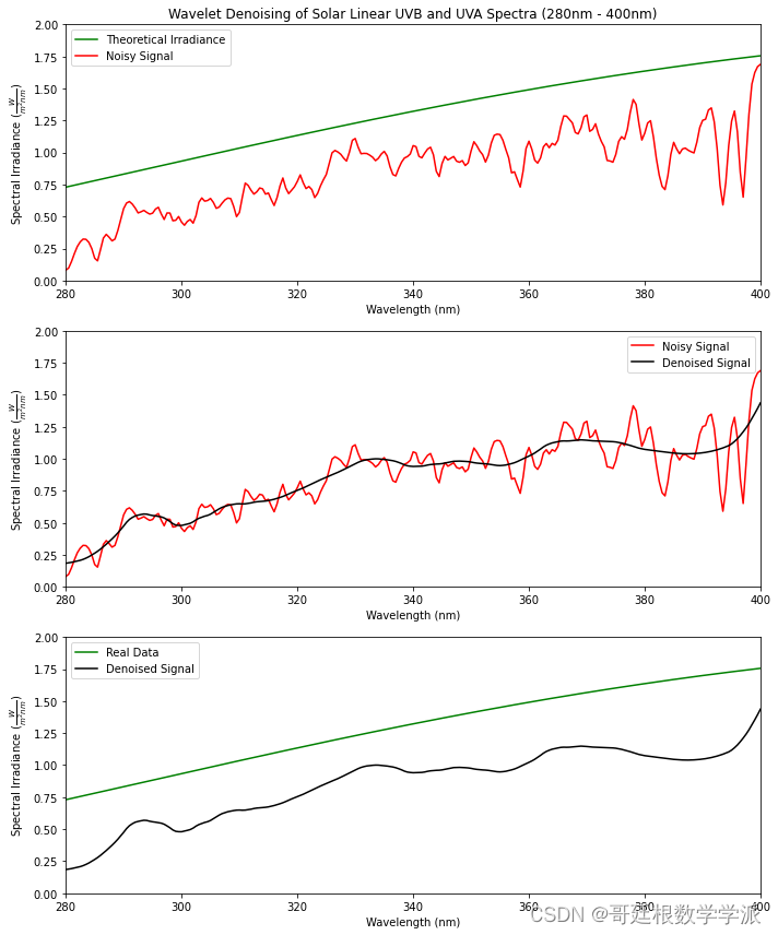
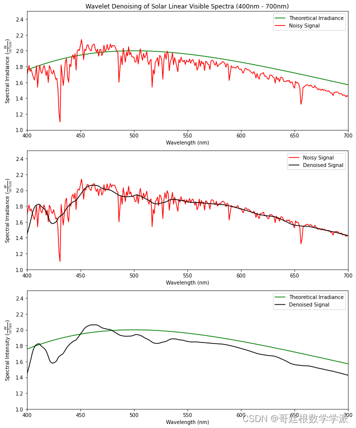
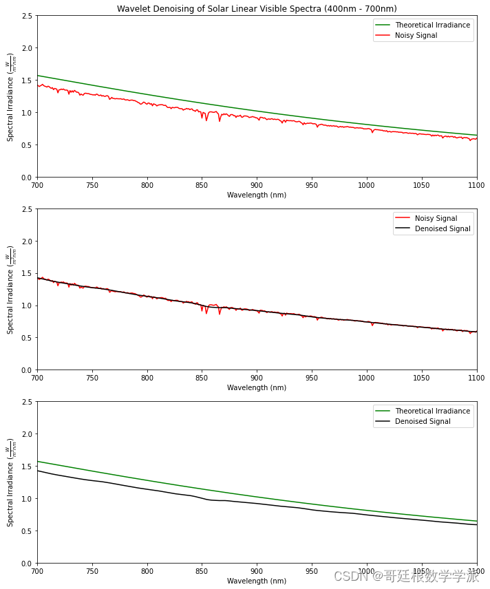
鉴于此，采用小波分析对电磁谱信号进行降噪，完整代码如下：

import numpy as npimport matplotlib.pyplot as pltimport pywtfrom scipy import constants as consdata = open('Data.txt', 'r')
wl = []intensity = []
for line in data:    rows = [i for i in line.split()]    wl.append(float(rows[0]))    intensity.append(float(rows[1]))
h = 6.626e-34  # Planck's constant (J·s)c = 3e8       # Speed of light (m/s)k = 1.381e-23  # Boltzmann constant (J/K)temperature = 5800  # Temperature (K)wien_constant = 2.897e-3  # Wien's displacement constant (m/K)
desired_peak = 2
# Wavelength range (in meters)wavelengths = np.linspace(280, 1100, 941) * 1e-9
# Planck's law for spectral radiancedef planck_law(wavelength, temperature):    return (8 * np.pi * h * c) / (wavelength**5) / (np.exp((h * c) / (wavelength * k * temperature)) - 1)
# Calculate spectral radiance for the Sunspectral_irradiance = planck_law(wavelengths, temperature)
# Normalize to have the peak value equal to the desired valuescaling_factor = desired_peak / np.max(spectral_irradiance)spectral_irradiance *= scaling_factor
peak_wavelength = 1e9*wien_constant / temperaturepeak_wavelength
DWTcoeffs = pywt.wavedec(intensity, 'db4')DWTcoeffs[-1] = np.zeros_like(DWTcoeffs[-1])DWTcoeffs[-2] = np.zeros_like(DWTcoeffs[-2])DWTcoeffs[-3] = np.zeros_like(DWTcoeffs[-3])DWTcoeffs[-4] = np.zeros_like(DWTcoeffs[-4])#DWTcoeffs[-5] = np.zeros_like(DWTcoeffs[-5])#DWTcoeffs[-6] = np.zeros_like(DWTcoeffs[-6])#DWTcoeffs[-7] = np.zeros_like(DWTcoeffs[-7])#DWTcoeffs[-8] = np.zeros_like(DWTcoeffs[-8])#DWTcoeffs[-9] = np.zeros_like(DWTcoeffs[-9])
filtered_data=pywt.waverec(DWTcoeffs,'db4')filtered_data = filtered_data[:len(wl)]
plt.figure(figsize=(10, 6))plt.plot(wavelengths * 1e9, spectral_irradiance, color='green', label='Theoretical Irradiance')plt.plot(wl, intensity, color='red', label='Noisy Signal')plt.plot(wl, filtered_data,  markerfacecolor='none',color='black', label='Denoised Signal')
plt.annotate(    str(temperature)+' K BlackBody Spectrum',    ha = 'center', va = 'bottom',    xytext = (900,1.75),    xy = (700,1.60),    arrowprops = { 'facecolor' : 'black', 'shrink' : 0.05 })
plt.legend()plt.title('Wavelet Denoising of Solar Linear Spectra (280nm - 1100nm)')plt.xlabel(r'Wavelength (nm)')plt.ylabel(r'Spectral Irradiance $(\frac{W}{m^2nm})$')plt.axis([280, 1100, 0, 2.5])plt.show()
plt.figure(figsize=(10, 12))  # Set the figure size for both subplots
# Subplot 1plt.subplot(3, 1, 1)  # Three rows, one column, index 1plt.plot(wavelengths * 1e9, spectral_irradiance, color='green', label='Theoretical Irradiance')plt.plot(wl, intensity, color='red', label='Noisy Signal')plt.legend()plt.title('Wavelet Denoising of Solar Linear UVB and UVA Spectra (280nm - 400nm)')plt.xlabel(r'Wavelength (nm)')plt.ylabel(r'Spectral Irradiance $(\frac{W}{m^2nm})$')plt.axis([280, 400, 0, 2])
# Subplot 2plt.subplot(3, 1, 2)  # Three rows, one column, index 2plt.plot(wl, intensity, color='red', label='Noisy Signal')plt.plot(wl, filtered_data, markerfacecolor='none', color='black', label='Denoised Signal')plt.legend()plt.xlabel(r'Wavelength (nm)')plt.ylabel(r'Spectral Irradiance $(\frac{W}{m^2nm})$')plt.axis([280, 400, 0, 2])
# Subplot 2plt.subplot(3, 1, 3)  # Three rows, one column, index 3plt.plot(wavelengths * 1e9, spectral_irradiance, color='green', label='Real Data')plt.plot(wl, filtered_data, markerfacecolor='none', color='black', label='Denoised Signal')plt.legend()plt.xlabel(r'Wavelength (nm)')plt.ylabel(r'Spectral Irradiance $(\frac{W}{m^2nm})$')plt.axis([280, 400, 0, 2])
plt.tight_layout()  # Adjust layout to prevent overlappingplt.show()
plt.figure(figsize=(10, 12))  # Set the figure size for both subplots
# Subplot 1plt.subplot(3, 1, 1)  # Three rows, one column, index 1plt.plot(wavelengths * 1e9, spectral_irradiance, color='green', label='Theoretical Irradiance')plt.plot(wl, intensity, color='red', label='Noisy Signal')plt.legend()plt.title('Wavelet Denoising of Solar Linear Visible Spectra (400nm - 700nm)')plt.xlabel(r'Wavelength (nm)')plt.ylabel(r'Spectral Irradiance $(\frac{W}{m^2nm})$')plt.axis([400, 700, 1, 2.5])
# Subplot 2plt.subplot(3, 1, 2)  # Three rows, one column, index 2plt.plot(wl, intensity, color='red', label='Noisy Signal')plt.plot(wl, filtered_data, markerfacecolor='none', color='black', label='Denoised Signal')plt.legend()plt.xlabel(r'Wavelength (nm)')plt.ylabel(r'Spectral Irradiance $(\frac{W}{m^2nm})$')plt.axis([400, 700, 1, 2.5])
# Subplot 2plt.subplot(3, 1, 3)  # Three rows, one column, index 3plt.plot(wavelengths * 1e9, spectral_irradiance, color='green', label='Theoretical Irradiance')plt.plot(wl, filtered_data, markerfacecolor='none', color='black', label='Denoised Signal')plt.legend()plt.xlabel(r'Wavelength (nm)')plt.ylabel(r'Spectral Intensity $(\frac{W}{m^2nm})$')plt.axis([400, 700, 1, 2.5])
plt.tight_layout()  # Adjust layout to prevent overlappingplt.show()
plt.figure(figsize=(10, 12))  # Set the figure size for both subplots
# Subplot 1plt.subplot(3, 1, 1)  # Three rows, one column, index 1plt.plot(wavelengths * 1e9, spectral_irradiance, color='green', label='Theoretical Irradiance')plt.plot(wl, intensity, color='red', label='Noisy Signal')plt.legend()plt.title('Wavelet Denoising of Solar Linear Visible Spectra (400nm - 700nm)')plt.xlabel(r'Wavelength (nm)')plt.ylabel(r'Spectral Irradiance $(\frac{W}{m^2nm})$')plt.axis([700, 1100, 0, 2.5])
# Subplot 2plt.subplot(3, 1, 2)  # Three rows, one column, index 2plt.plot(wl, intensity, color='red', label='Noisy Signal')plt.plot(wl, filtered_data, markerfacecolor='none', color='black', label='Denoised Signal')plt.legend()plt.xlabel(r'Wavelength (nm)')plt.ylabel(r'Spectral Irradiance $(\frac{W}{m^2nm})$')plt.axis([700, 1100, 0, 2.5])
# Subplot 2plt.subplot(3, 1, 3)  # Three rows, one column, index 3plt.plot(wavelengths * 1e9, spectral_irradiance, color='green', label='Theoretical Irradiance')plt.plot(wl, filtered_data, markerfacecolor='none', color='black', label='Denoised Signal')plt.legend()plt.xlabel(r'Wavelength (nm)')plt.ylabel(r'Spectral Irradiance $(\frac{W}{m^2nm})$')plt.axis([700, 1100, 0, 2.5])
plt.tight_layout()  # Adjust layout to prevent overlappingplt.show()
def calculate_mse(original, denoised):    mse = np.mean(np.square(np.subtract(original, denoised)))    return mse
def calculate_rmse(original, denoised):    mse = calculate_mse(original, denoised)    rmse = np.sqrt(mse)    return rmse
def calculate_psnr(original, denoised):    max_pixel_value = 255.0  # Assuming pixel values are in the range [0, 255]    mse_value = calculate_mse(original, denoised)    psnr = 10 * np.log10((max_pixel_value ** 2) / mse_value)    return psnr
# Assuming 'original_signal' and 'denoised_signal' are your original and denoised signals as lists or arraysmse_value = calculate_mse(spectral_irradiance, filtered_data)rmse_value = calculate_rmse(spectral_irradiance, filtered_data)psnr_value = calculate_psnr(spectral_irradiance, filtered_data)
print(f"MSE: {mse_value}")print(f"RMSE: {rmse_value}")print(f"PSNR: {psnr_value} dB")