Jupyter Notebook 代码连接:
machine_learning_demo
machine_learning_ensembles
Step 1: Imports and Configuration
import pandas as pd
import numpy as np
import copy
import json
import pickle
import joblib
import lightgbm as lgb
import optuna
import warnings
import gcfrom sklearn.metrics import roc_curve, roc_auc_score, recall_score, accuracy_score, fbeta_score, precision_score
from sklearn.model_selection import train_test_split, cross_val_score, KFold
from sklearn.base import clone
import matplotlib.pyplot as plt
import seaborn as sns# Setting configuration.
pd.set_option('display.float_format', lambda x: '%.5f' %x)
warnings.filterwarnings('ignore')
sns.set_style('whitegrid')
optuna.logging.set_verbosity(optuna.logging.WARNING)SEED = 42
Step 2: Load the datasets
print('Loading data...')
path = '../datasets/Home-Credit-Default-Risk/'
df = pd.read_csv(path + 'selected_data.csv', index_col='SK_ID_CURR')
Loading data...
定义帮助节省内存的函数
def convert_dtypes(df, verbose=True):original_memory = df.memory_usage().sum()df = df.apply(pd.to_numeric, errors='ignore')# Convert booleans to integersboolean_features = df.select_dtypes(bool).columns.tolist()df[boolean_features] = df[boolean_features].astype(np.int32)# Convert objects to categoryobject_features = df.select_dtypes(object).columns.tolist()df[object_features] = df[object_features].astype('category')# Float64 to float32float_features = df.select_dtypes(float).columns.tolist()df[float_features] = df[float_features].astype(np.float32)# Int64 to int32int_features = df.select_dtypes(int).columns.tolist()df[int_features] = df[int_features].astype(np.int32)new_memory = df.memory_usage().sum()if verbose:print(f'Original Memory Usage: {round(original_memory / 1e9, 2)} gb.')print(f'New Memory Usage: {round(new_memory / 1e9, 2)} gb.')return df
print("Training dataset shape: ", df.shape)
Training dataset shape: (307511, 836)
df = convert_dtypes(df)
Original Memory Usage: 2.06 gb.
New Memory Usage: 1.0 gb.
df.dtypes.value_counts()
float32     796
int32         7
category      3
category      3
category      3
category      3
category      3
category      2
category      2
category      2
category      1
category      1
category      1
category      1
category      1
category      1
category      1
category      1
category      1
category      1
category      1
category      1
Name: count, dtype: int64
Step 3: Data preprocessing
# Check if the data is unbalanced
df["TARGET"].value_counts()
TARGET
0    282686
1     24825
Name: count, dtype: int64
数据集存在轻微的样本不平衡,我们接下来测试几种处理方法,来提高模型表现。
先定义评估函数
def timer(func):import timeimport functoolsdef strfdelta(tdelta, fmt):hours, remainder = divmod(tdelta, 3600)minutes, seconds = divmod(remainder, 60)return fmt.format(hours, minutes, seconds)@functools.wraps(func)def wrapper(*args, **kwargs):click = time.time()result = func(*args, **kwargs)delta = strfdelta(time.time() - click, "{:.0f} hours {:.0f} minutes {:.0f} seconds")print(f"{func.__name__} cost time {delta}")return resultreturn wrapper# Define a cross validation strategy
# We use the cross_val_score function of Sklearn.
# However this function has not a shuffle attribute, we add then one line of code,
# in order to shuffle the dataset prior to cross-validation@timer
def evaluate(model, X, y, n_folds = 5, params=None):kf = KFold(n_folds, shuffle=True, random_state=SEED).get_n_splits(X)scores = cross_val_score(model, X, y, scoring="roc_auc", cv = kf,verbose=1,params=params)print(f"valid auc: {scores.mean():.3f} +/- {scores.std():.3f}")return scores.mean()
Split data
留25%作为模型的验证集
# Split data into training and testing sets
X_train, X_valid, y_train, y_valid = train_test_split(df.drop(columns="TARGET"), df["TARGET"], test_size=0.25, random_state=SEED
)print("X_train shape:", X_train.shape)
print('train:', y_train.value_counts(), sep='\n')
print('valid:', y_valid.value_counts(), sep='\n')
X_train shape: (230633, 835)
train:
TARGET
0    211999
1     18634
Name: count, dtype: int64
valid:
TARGET
0    70687
1     6191
Name: count, dtype: int64
del df
gc.collect()
# Specific feature names and categorical features
feature_name = X_train.columns.tolist()
categorical_feature = X_train.select_dtypes('category').columns.tolist()
from sklearn.preprocessing import OneHotEncoder
from sklearn.compose import make_column_transformer# Encode categorical features
encoder = make_column_transformer((OneHotEncoder(drop='if_binary', min_frequency=0.02, max_categories=20, sparse_output=False,handle_unknown='ignore'), categorical_feature),remainder='passthrough', verbose_feature_names_out=False,verbose=True
)print('fitting...')
encoder.fit(X_train)print('encoding...')
train_dummies = encoder.transform(X_train)
valid_dummies = encoder.transform(X_valid)
print('train data shape:', X_train.shape)
fitting...
[ColumnTransformer] . (1 of 2) Processing onehotencoder, total=   4.2s
[ColumnTransformer] ..... (2 of 2) Processing remainder, total=   0.0s
encoding...
train data shape: (230633, 835)
model 1: Use default parameters
model = lgb.LGBMClassifier(boosting_type='gbdt',objective='binary',metric='auc',n_estimators=500,random_state=SEED,verbose=0
)
fit_params = dict(callbacks = [lgb.early_stopping(20)],eval_set = [(train_dummies, y_train), (valid_dummies, y_valid)]
)score = evaluate(model, train_dummies, y_train, params=fit_params)
Training until validation scores don't improve for 20 rounds
Early stopping, best iteration is:
[147]	valid_0's auc: 0.860844	valid_1's auc: 0.778985
Training until validation scores don't improve for 20 rounds
Early stopping, best iteration is:
[99]	valid_0's auc: 0.836905	valid_1's auc: 0.777066
Training until validation scores don't improve for 20 rounds
Early stopping, best iteration is:
[121]	valid_0's auc: 0.846901	valid_1's auc: 0.777927
Training until validation scores don't improve for 20 rounds
Early stopping, best iteration is:
[118]	valid_0's auc: 0.846341	valid_1's auc: 0.778487
Training until validation scores don't improve for 20 rounds
Early stopping, best iteration is:
[114]	valid_0's auc: 0.845653	valid_1's auc: 0.776624
valid auc: 0.779 +/- 0.001
evaluate cost time 0 hours 1 minutes 57 seconds
model 2: Set class weight
model2 = clone(model) # Construct a new unfitted estimator with the same parameters.
model2.set_params(class_weight='balanced')score = evaluate(model2, train_dummies, y_train, params=fit_params)
Training until validation scores don't improve for 20 rounds
Early stopping, best iteration is:
[122]	valid_0's auc: 0.843105	valid_1's auc: 0.780157
Training until validation scores don't improve for 20 rounds
Early stopping, best iteration is:
[95]	valid_0's auc: 0.831016	valid_1's auc: 0.780049
Training until validation scores don't improve for 20 rounds
Early stopping, best iteration is:
[107]	valid_0's auc: 0.835709	valid_1's auc: 0.779769
Training until validation scores don't improve for 20 rounds
Early stopping, best iteration is:
[159]	valid_0's auc: 0.856821	valid_1's auc: 0.781057
Training until validation scores don't improve for 20 rounds
Early stopping, best iteration is:
[138]	valid_0's auc: 0.848312	valid_1's auc: 0.779905
valid auc: 0.780 +/- 0.002
evaluate cost time 0 hours 2 minutes 20 seconds
设置 is_unbalance=True 后,模型有所改善。
model 3: SMOTE
from imblearn.over_sampling import SMOTE
import imblearnX_balanced, y_balanced = SMOTE(random_state=SEED).fit_resample(train_dummies, y_train)
print('balanced train data shape:', X_balanced.shape)score = evaluate(clone(model), X_balanced, y_balanced, params=fit_params)
balanced train data shape: (423998, 990)
Training until validation scores don't improve for 20 rounds
Early stopping, best iteration is:
[64]	valid_0's auc: 0.726936	valid_1's auc: 0.7216
Training until validation scores don't improve for 20 rounds
Early stopping, best iteration is:
[138]	valid_0's auc: 0.834743	valid_1's auc: 0.780546
Training until validation scores don't improve for 20 rounds
Early stopping, best iteration is:
[167]	valid_0's auc: 0.849441	valid_1's auc: 0.782093
Training until validation scores don't improve for 20 rounds
Early stopping, best iteration is:
[140]	valid_0's auc: 0.834219	valid_1's auc: 0.780796
Training until validation scores don't improve for 20 rounds
Early stopping, best iteration is:
[166]	valid_0's auc: 0.848353	valid_1's auc: 0.780799
valid auc: 0.976 +/- 0.048
evaluate cost time 0 hours 5 minutes 46 seconds
model 4: Ensemble method
from imblearn.ensemble import BalancedRandomForestClassifiermodel4 = BalancedRandomForestClassifier(n_estimators=100, max_depth=5,random_state=SEED,verbose=1
)
score = evaluate(model4, train_dummies, y_train)
[Parallel(n_jobs=1)]: Done  49 tasks      | elapsed:    7.3s
[Parallel(n_jobs=1)]: Done  49 tasks      | elapsed:    0.1s
[Parallel(n_jobs=1)]: Done  49 tasks      | elapsed:    7.2s
[Parallel(n_jobs=1)]: Done  49 tasks      | elapsed:    0.1s
[Parallel(n_jobs=1)]: Done  49 tasks      | elapsed:    7.2s
[Parallel(n_jobs=1)]: Done  49 tasks      | elapsed:    0.2s
[Parallel(n_jobs=1)]: Done  49 tasks      | elapsed:    7.3s
[Parallel(n_jobs=1)]: Done  49 tasks      | elapsed:    0.2s
[Parallel(n_jobs=1)]: Done  49 tasks      | elapsed:    7.1s
[Parallel(n_jobs=1)]: Done  49 tasks      | elapsed:    0.1svalid auc: 0.738 +/- 0.002
evaluate cost time 0 hours 1 minutes 21 seconds
model 5: FocalLoss
from focal_loss import BinaryFocalLoss # self-define loss functionfocalloss = BinaryFocalLoss(alpha=0.9, gamma=0.05)
model5 = clone(model)
model5.set_params(objective = focalloss.objective)
fit_params['eval_metric'] = focalloss.evaluatescore = evaluate(model5, train_dummies, y_train, params=fit_params)
[LightGBM] [Info] Using self-defined objective function
Training until validation scores don't improve for 20 rounds
Early stopping, best iteration is:
[116]	valid_0's auc: 0.840709	valid_0's focal_loss: 0.0792912	valid_1's auc: 0.780966	valid_1's focal_loss: 0.0886921
[LightGBM] [Info] Using self-defined objective function
Training until validation scores don't improve for 20 rounds
Early stopping, best iteration is:
[87]	valid_0's auc: 0.82691	valid_0's focal_loss: 0.0816416	valid_1's auc: 0.779874	valid_1's focal_loss: 0.0888508
[LightGBM] [Info] Using self-defined objective function
Training until validation scores don't improve for 20 rounds
Early stopping, best iteration is:
[101]	valid_0's auc: 0.832985	valid_0's focal_loss: 0.0805644	valid_1's auc: 0.779294	valid_1's focal_loss: 0.0889485
[LightGBM] [Info] Using self-defined objective function
Training until validation scores don't improve for 20 rounds
Early stopping, best iteration is:
[87]	valid_0's auc: 0.827538	valid_0's focal_loss: 0.0816012	valid_1's auc: 0.78189	valid_1's focal_loss: 0.0885146
[LightGBM] [Info] Using self-defined objective function
Training until validation scores don't improve for 20 rounds
Early stopping, best iteration is:
[119]	valid_0's auc: 0.840904	valid_0's focal_loss: 0.0792486	valid_1's auc: 0.781548	valid_1's focal_loss: 0.0886565
valid auc: nan +/- nan
evaluate cost time 0 hours 2 minutes 16 seconds
自定义FocalLoss损失函数后,表现不错
del train_dummies, valid_dummies
gc.collect()
Step 4: Hyperparameter Tuning
超参数调优算法主要有网格搜索(Grid Search),随机搜索(Randomized Search)和贝叶斯优化(Bayesian Optimization),本文采用贝叶斯优化。
本章准备使用LightGBM原生接口,需要创建 lightgbm 原生数据集
# Create Dataset object for lightgbm
dtrain = lgb.Dataset(X_train, label=y_train, free_raw_data=True
)# In LightGBM, the validation data should be aligned with training data.
# if you want to re-use data, remember to set free_raw_data=False
dvalid = lgb.Dataset(X_valid, label=y_valid, reference=dtrain, free_raw_data=True
)
超参数和目标函数设置
# Here we use Optuna# define the search space and the objecive function
def objective(trial):# LightGBM can use a dictionary to set Parameters.params = dict(boosting_type = 'gbdt',objective = 'binary',metric = 'auc',is_unbalance = True,num_boost_round = trial.suggest_int("num_boost_round", 50, 2000, step=50),learning_rate = trial.suggest_float("learning_rate", 1e-4, 10, log=True), max_depth = trial.suggest_int("max_depth", 2, 10),  feature_fraction = trial.suggest_float("feature_fraction", 0.2, 1.0), bagging_fraction = trial.suggest_float("bagging_fraction", 0.2, 1.0),  bagging_freq = 5,lambda_l1 = trial.suggest_float("lambda_l1", 1e-4, 1e2, log=True),  lambda_l2 = trial.suggest_float("lambda_l2", 1e-4, 1e2, log=True),random_state = SEED,verbosity = -1)# Perform the cross-validation with given parameters.eval_results = lgb.cv(params, dtrain, nfold = 5,shuffle = True,feature_name = feature_name,categorical_feature = categorical_feature,callbacks=[lgb.early_stopping(20)])return eval_results['valid auc-mean'][-1]
贝叶斯优化
# Bayesian optimization# create a study object.
study = optuna.create_study(study_name = 'lightgbm-study',  # Unique identifier of the study.direction = 'maximize'
)# Invoke optimization of the objective function.
study.optimize(objective, n_trials = 100, timeout = 7200,gc_after_trial = True,show_progress_bar = True
)
joblib.dump(study, path + "lightgbm-study.pkl")study = joblib.load(path + "lightgbm-study.pkl")print("Best trial until now:")
print(" Value: ", study.best_trial.value)
print(" Params: ")
for key, value in study.best_trial.params.items():print(f"    {key}: {value}")
Best trial until now:Value: 0.785777090367696Params: num_boost_round: 1000learning_rate: 0.029182324488925142max_depth: 8feature_fraction: 0.902981862669475bagging_fraction: 0.9853966386414182lambda_l1: 73.55650874339202lambda_l2: 6.572289325673235
# Continue to study
study.optimize(objective, n_trials = 100, timeout = 7200,gc_after_trial = True,show_progress_bar = True
)
print("Number of finished trials: ", len(study.trials))
print("Best trial until now:")
print(" Best value: ", study.best_trial.value)
print(" Best params: ")
for key, value in study.best_trial.params.items():print(f"    {key}: {value}")
Number of finished trials:  135
Best trial until now:Best value:  0.7865747325768904Best params: num_boost_round: 1300learning_rate: 0.015480784915810246max_depth: 8feature_fraction: 0.3519165350962246bagging_fraction: 0.9999568798413535lambda_l1: 65.08840723355036lambda_l2: 15.024421566966097
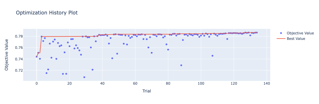
可视化
绘制优化过程曲线
optuna.visualization.plot_optimization_history(study)
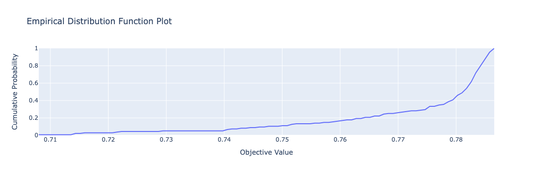
绘制study目标值的edf
optuna.visualization.plot_edf(study)
Step 5: Training
训练
本节准备使用LightGBM原生接口,需要创建 lightgbm 原生数据集
# Create Dataset object for lightgbm
dtrain = lgb.Dataset(X_train, label=y_train, free_raw_data=True
)# In LightGBM, the validation data should be aligned with training data.
# if you want to re-use data, remember to set free_raw_data=False
dvalid = lgb.Dataset(X_valid, label=y_valid, reference=dtrain, free_raw_data=True)
print('Starting training...')best_params = dict(boosting_type = 'gbdt',objective = 'binary',metric = 'auc',is_unbalance = True,num_boost_round = 1300,learning_rate = 0.015480784915810246,max_depth = 8,feature_fraction = 0.3519165350962246,bagging_fraction = 0.9999568798413535,lambda_l1 = 65.08840723355036,lambda_l2 = 15.024421566966097,subsample_freq = 5,random_state = SEED,verbosity = 0
)eval_results = {} # to record eval results for plotting
callbacks = [lgb.log_evaluation(period=100), lgb.early_stopping(stopping_rounds=20),lgb.record_evaluation(eval_results)
]# Training
bst = lgb.train(best_params, dtrain, feature_name = feature_name, categorical_feature = categorical_feature,valid_sets = [dtrain, dvalid],callbacks = callbacks
)
Starting training...
[LightGBM] [Warning] Accuracy may be bad since you didn't explicitly set num_leaves OR 2^max_depth > num_leaves. (num_leaves=31).
[LightGBM] [Warning] Accuracy may be bad since you didn't explicitly set num_leaves OR 2^max_depth > num_leaves. (num_leaves=31).
[LightGBM] [Warning] Found whitespace in feature_names, replace with underlines
[LightGBM] [Warning] Accuracy may be bad since you didn't explicitly set num_leaves OR 2^max_depth > num_leaves. (num_leaves=31).
[LightGBM] [Warning] Accuracy may be bad since you didn't explicitly set num_leaves OR 2^max_depth > num_leaves. (num_leaves=31).
[LightGBM] [Warning] Found whitespace in feature_names, replace with underlines
[LightGBM] [Warning] Accuracy may be bad since you didn't explicitly set num_leaves OR 2^max_depth > num_leaves. (num_leaves=31).
Training until validation scores don't improve for 20 rounds
[100]	training's auc: 0.77831	valid_1's auc: 0.760952
[200]	training's auc: 0.793115	valid_1's auc: 0.770076
[300]	training's auc: 0.803729	valid_1's auc: 0.775631
[400]	training's auc: 0.811797	valid_1's auc: 0.778893
[500]	training's auc: 0.818789	valid_1's auc: 0.78126
[600]	training's auc: 0.825071	valid_1's auc: 0.782986
[700]	training's auc: 0.830958	valid_1's auc: 0.784242
[800]	training's auc: 0.836567	valid_1's auc: 0.785216
[900]	training's auc: 0.841761	valid_1's auc: 0.785837
[1000]	training's auc: 0.846603	valid_1's auc: 0.786335
[1100]	training's auc: 0.851281	valid_1's auc: 0.786744
Early stopping, best iteration is:
[1118]	training's auc: 0.852112	valid_1's auc: 0.786804
可视化
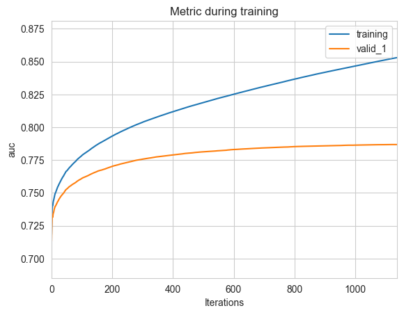
# Plotting metrics recorded during training
ax = lgb.plot_metric(eval_results, metric='auc')
plt.show()
Step 6: Evaluating
模型得分
def get_adjusted_prediction(y_score, threshold=0.5):y_pred = y_score.copy()y_pred[y_score>=threshold] = 1y_pred[y_score< threshold] = 0return y_preddef classification_report(model, X, y):from sklearn.metrics import balanced_accuracy_scorereport = {}y_true = yy_score = model.predict(X) if y_score.ndim >= 2:y_pred = np.argmax(y_score)else:y_pred = (y_score > 0.5).astype(int)fpr, tpr, thresholds = roc_curve(y_true, y_score) idx = (tpr - fpr).argmax()adjusted_threshold = thresholds[idx]adjusted_y_pred = (y_score > adjusted_threshold).astype(int) return {'y_pred': y_pred,'y_score': y_score,'fpr': fpr,'tpr': tpr, 'thresholds': thresholds,'ks': (tpr - fpr).max(),'auc': roc_auc_score(y_true, y_score),'accuracy': accuracy_score(y_true, y_pred),'balanced_accuracy_score': balanced_accuracy_score(y_true, y_pred),'precision': precision_score(y_true, y_pred),'recall': recall_score(y_true, y_pred),'f1-score': fbeta_score(y_true, y_pred, beta=1),'adjusted_threshold': adjusted_threshold,'adjusted_accuracy': accuracy_score(y_true, adjusted_y_pred)}
# the model performance
train_report = classification_report(bst, X_train, y_train)
valid_report = classification_report(bst, X_valid, y_valid)
for label, stats in [('train data', train_report), ('valid data', valid_report)]:print(label, ":")print(f"auc: {stats['auc']:.5f}", f"accuracy: {stats['accuracy']:.5f}", f"balanced_accuracy_score: {stats['balanced_accuracy_score']:.5f}",f"adjusted_accuracy(threshold = {stats['adjusted_threshold']:.4f}): {stats['adjusted_accuracy']:.5f}", f"recall: {stats['recall']:.5f}", sep = '\n\t')
train data :
auc: 0.85211accuracy: 0.75527balanced_accuracy_score: 0.77060adjusted_accuracy(threshold = 0.4885): 0.74530recall: 0.78888
valid data :
auc: 0.78680accuracy: 0.73706balanced_accuracy_score: 0.71237adjusted_accuracy(threshold = 0.4526): 0.69454recall: 0.68293
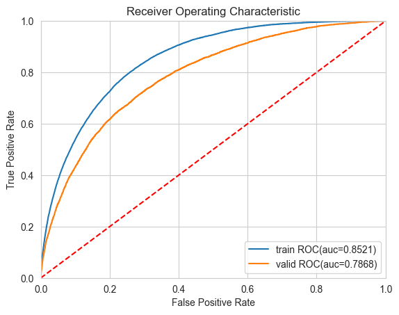
ROC曲线
# Plot ROC curve
def plot_roc_curve(fprs, tprs, labels):from sklearn import metricsplt.figure()plt.title('Receiver Operating Characteristic')plt.xlabel('False Positive Rate')plt.ylabel('True Positive Rate')plt.plot([0, 1], [0, 1],'r--')plt.xlim([0, 1])plt.ylim([0, 1])# Plotting ROC and computing AUC scoresfor fpr, tpr, label in zip(fprs, tprs, labels):auc = metrics.auc(fpr, tpr)plt.plot(fpr, tpr, label = f"{label} ROC(auc={auc:.4f})")plt.legend(loc = 'lower right')plot_roc_curve(fprs = (train_report['fpr'], valid_report['fpr']),tprs = (train_report['tpr'], valid_report['tpr']),labels = ('train', 'valid')
)
模型稳定性
PSI(Population Stability Index)指标反映了实际分布(actual)与预期分布(expected)的差异。在建模中,我们常用来筛选特征变量、评估模型稳定性。其中,在建模时通常以训练样本(In the Sample, INS)作为预期分布,而验证样本在各分数段的分布通常作为实际分布。验证样本一般包括样本外(Out of Sample, OOS)和跨时间样本(Out of Time, OOT)。
风控模型常用PSI衡量模型的稳定性。
def calc_psi(expected, actual, n_bins=10):'''Calculate the PSI (Population Stability Index) for two vectors.Args:expected: array-like, represents the expected distribution.actual: array-like, represents the actual distribution.bins: int, the number of bins to use in the histogram.Returns:float, the PSI value.'''# Calculate the expected frequencies in each binbuckets, bins = pd.qcut(expected, n_bins, retbins=True, duplicates='drop')expected_freq = buckets.value_counts() expected_freq = expected_freq / expected_freq.sum()# Calculate the actual frequencies in each binbins = [-np.inf] + list(bins)[1: -1] + [np.inf]actual_freq = pd.cut(actual, bins).value_counts()actual_freq = actual_freq / actual_freq.sum()# Calculate PSIpsi = (actual_freq - expected_freq) * np.log(actual_freq / expected_freq)return psi.sum()psi = calc_psi(train_report['y_score'], valid_report['y_score'])
print("PSI:", psi)
PSI: 0.00019890720303521737
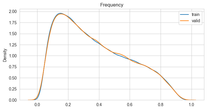
绘制实际分布与预期分布曲线
plt.figure(figsize=(8, 4))
sns.kdeplot(x=train_report['y_score'], label='train')
sns.kdeplot(x=valid_report['y_score'], label='valid')
plt.legend(loc='best')
plt.title(label = 'Frequency', loc ='center')
验证集正负样本分布曲线
valid_pred = pd.DataFrame({'score': valid_report['y_score'], 'target': y_valid})plt.figure(figsize=(8, 4))
sns.kdeplot(data=valid_pred, x='score', hue='target', common_norm=False)
plt.title(label = 'Frequency', loc ='center')

验证集正负样本累积分布
plt.figure(figsize=(8, 4))
sns.kdeplot(data=valid_pred, x='score', hue='target', common_norm=False, cumulative=True)
plt.title(label = 'Cumulative', loc ='center')

Step 7: Show feature importance
feature_imp = pd.Series(bst.feature_importance(), index=bst.feature_name()
).sort_values(ascending=False)print(feature_imp.head(20))
feature_imp.to_excel(path + 'feature_importance.xlsx')
AMT_ANNUITY_/_AMT_CREDIT                           776
MODE(previous.PRODUCT_COMBINATION)                 590
MODE(installments.previous.PRODUCT_COMBINATION)    475
MODE(cash.previous.PRODUCT_COMBINATION)            355
EXT_SOURCE_2_+_EXT_SOURCE_3                        312
MAX(bureau.DAYS_CREDIT_ENDDATE)                    296
MAX(bureau.DAYS_CREDIT)                            281
MODE(previous.NAME_GOODS_CATEGORY)                 274
MODE(installments.previous.NAME_GOODS_CATEGORY)    270
MEAN(bureau.AMT_CREDIT_SUM_DEBT)                   252
MODE(cash.previous.NAME_GOODS_CATEGORY)            248
AMT_GOODS_PRICE_/_AMT_ANNUITY                      232
MEAN(previous.MEAN(cash.CNT_INSTALMENT_FUTURE))    210
frequency(CODE_GENDER_M)_by(EXT_SOURCE_1)          196
AMT_CREDIT_-_AMT_GOODS_PRICE                       195
SUM(bureau.AMT_CREDIT_SUM)                         192
SUM(bureau.AMT_CREDIT_MAX_OVERDUE)                 191
EXT_SOURCE_1_/_DAYS_BIRTH                          182
MAX(cash.previous.DAYS_LAST_DUE_1ST_VERSION)       178
DAYS_BIRTH_/_EXT_SOURCE_1                          176
dtype: int32
# Plotting feature importances
ax = lgb.plot_importance(bst, max_num_features=20)
plt.show()

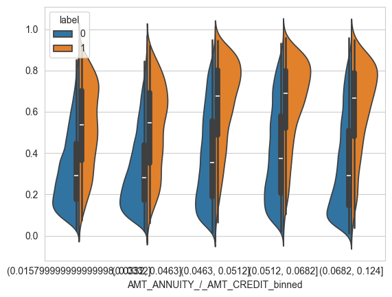
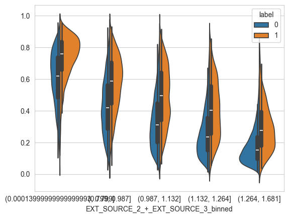
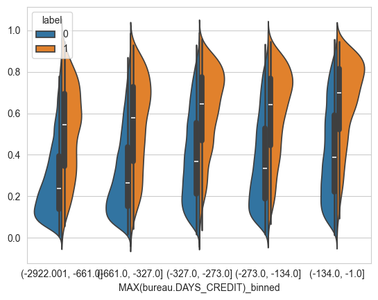
观察重点特征的分布
X_valid.columns = X_valid.columns.str.replace(' ', '_')for col in feature_imp.index[:10]:table = pd.DataFrame({col: X_valid[col], 'label': y_valid})if table[col].dtype in [np.float32, np.int32]:table[f'{col}_binned'] = pd.qcut(table[col], 5, duplicates='drop')else:table[f'{col}_binned'] = table[col] print(table.pivot_table(index=f'{col}_binned', columns='label',values='label',aggfunc='count'))if table[f'{col}_binned'].nunique() <= 5:sns.violinplot(data=table, x=f'{col}_binned',y=valid_report['y_score'],hue='label',split=True)plt.show()
label                                0     1
AMT_ANNUITY_/_AMT_CREDIT_binned
(0.015799999999999998, 0.0332]   14353  1039
(0.0332, 0.0463]                 14392   974
(0.0463, 0.0512]                 13906  1499
(0.0512, 0.0682]                 13890  1450
(0.0682, 0.124]                  14146  1229
label                                          0     1
MODE(previous.PRODUCT_COMBINATION)_binned
Card Street                                 6497   729
Card X-Sell                                 3161   274
Cash                                       12431  1234
Cash Street: high                           2147   240
Cash Street: low                             918    81
Cash Street: middle                          910    91
Cash X-Sell: high                           1695   207
Cash X-Sell: low                            2944   169
Cash X-Sell: middle                         3851   323
POS household with interest                17801  1333
POS household without interest              3204   205
POS industry with interest                  4379   282
POS industry without interest                474    17
POS mobile with interest                    8690   875
POS mobile without interest                  685    54
POS other with interest                      816    73
POS others without interest                   84     4
label                                                   0     1
MODE(installments.previous.PRODUCT_COMBINATION)...
Card Street                                          4039   472
Card X-Sell                                          5686   628
Cash Street: high                                    2265   259
Cash Street: low                                      903    77
Cash Street: middle                                  1300   128
Cash X-Sell: high                                    2132   251
Cash X-Sell: low                                     4010   193
Cash X-Sell: middle                                  5394   394
POS household with interest                         19706  1657
POS household without interest                       5942   412
POS industry with interest                           6274   424
POS industry without interest                         828    31
POS mobile with interest                             9593  1032
POS mobile without interest                          1086    97
POS other with interest                              1369   127
POS others without interest                           160     9
label                                               0     1
MODE(cash.previous.PRODUCT_COMBINATION)_binned
Cash Street: high                                2695   340
Cash Street: low                                 1053    95
Cash Street: middle                              1554   171
Cash X-Sell: high                                2544   315
Cash X-Sell: low                                 4653   258
Cash X-Sell: middle                              6635   496
POS household with interest                     22600  1994
POS household without interest                   6767   494
POS industry with interest                       6970   493
POS industry without interest                     923    35
POS mobile with interest                        11399  1241
POS mobile without interest                      1219   112
POS other with interest                          1498   136
POS others without interest                       177    11
label                                   0     1
EXT_SOURCE_2_+_EXT_SOURCE_3_binned
(0.00013999999999999993, 0.799]     12583  2793
(0.799, 0.987]                      13994  1381
(0.987, 1.132]                      14411   965
(1.132, 1.264]                      14688   687
(1.264, 1.681]                      15011   365
label                                       0     1
MAX(bureau.DAYS_CREDIT_ENDDATE)_binned
(-41875.001, 80.0]                      14445   941
(80.0, 823.0]                           14358  1014
(823.0, 983.0]                          13918  1453
(983.0, 1735.0]                         13997  1399
(1735.0, 31199.0]                       13969  1384

label                               0     1
MAX(bureau.DAYS_CREDIT)_binned
(-2922.001, -661.0]             14554   825
(-661.0, -327.0]                14371  1031
(-327.0, -273.0]                13949  1408
(-273.0, -134.0]                14068  1326
(-134.0, -1.0]                  13745  1601
label                                          0     1
MODE(previous.NAME_GOODS_CATEGORY)_binned
Additional Service                            10     0
Audio/Video                                 6458   469
Auto Accessories                             467    42
Clothing and Accessories                    1541    89
Computers                                   5827   482
Construction Materials                      1432   104
Consumer Electronics                        5977   422
Direct Sales                                  29     5
Education                                     13     1
Fitness                                       17     1
Furniture                                   2578   143
Gardening                                    129     5
Homewares                                    242    15
Insurance                                      0     0
Jewelry                                      247    24
Medical Supplies                             256    10
Medicine                                     112     7
Mobile                                      9794   935
Office Appliances                             50     2
Other                                         49     5
Photo / Cinema Equipment                     550    56
Sport and Leisure                             79    13
Tourism                                       78     3
Vehicles                                     140    12
Weapon                                         5     0
XNA                                        34607  3346
label                                                   0     1
MODE(installments.previous.NAME_GOODS_CATEGORY)...
Additional Service                                      9     0
Animals                                                 1     0
Audio/Video                                          6092   497
Auto Accessories                                      347    51
Clothing and Accessories                             1604    88
Computers                                            6324   542
Construction Materials                               1571   121
Consumer Electronics                                 7279   562
Direct Sales                                           13     4
Education                                              14     1
Fitness                                                22     1
Furniture                                            3235   208
Gardening                                             175     7
Homewares                                             363    29
Insurance                                               0     0
Jewelry                                               238    29
Medical Supplies                                      400    17
Medicine                                              162     9
Mobile                                              10152  1046
Office Appliances                                      90     9
Other                                                 100     7
Photo / Cinema Equipment                             1115   103
Sport and Leisure                                     150    18
Tourism                                               106     4
Vehicles                                              261    28
Weapon                                                  6     0
XNA                                                 30858  2810
label                                        0     1
MEAN(bureau.AMT_CREDIT_SUM_DEBT)_binned
(-220213.42299999998, 0.0]               16805   994
(0.0, 39052.254]                         12066   886
(39052.254, 49487.143]                   13928  1448
(49487.143, 148125.9]                    13904  1471
(148125.9, 43650000.0]                   13984  1392

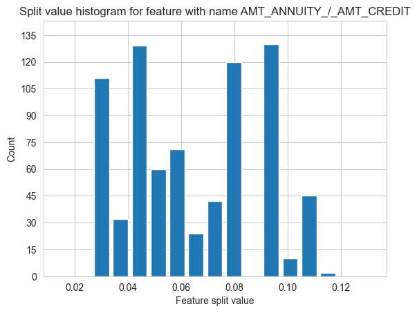
Step 8: Visualize the model
# Plotting split value histogram
ax = lgb.plot_split_value_histogram(bst, feature='AMT_ANNUITY_/_AMT_CREDIT', bins='auto')
plt.show()
# Plotting 54th tree (one tree use categorical feature to split)
# ax = lgb.plot_tree(bst, tree_index=53, figsize=(15, 15), show_info=['split_gain'])
# plt.show()# Plotting 54th tree with graphviz
# graph = lgb.create_tree_digraph(bst, tree_index=53, name='Tree54')
# graph.render(view=True)
Step 9: Model persistence
# Save model to file
print('Saving model...')
bst.save_model(path + 'lgb_model.txt')
Saving model...<lightgbm.basic.Booster at 0x2c457d3a0>
Step 10: Predict
# Perform predictions
# If early stopping is enabled during training, you can get predictions from the best iteration with bst.best_iteration.
predictions = bst.predict(X_valid, num_iteration=bst.best_iteration)
# Load a saved model to predict
print('Loading model to predict...')
bst = lgb.Booster(model_file=path + 'lgb_model.txt')
predictions = bst.predict(X_valid)
Loading model to predict...
# Save predictions
# predictions.to_csv('valid_predictions.csv', index=True)
Appendices: FocalLoss
import numpy as np
from scipy import optimize, specialclass BinaryFocalLoss:def __init__(self, gamma, alpha=None):# 使用FocalLoss只需要设定以上两个参数,如果alpha=None,默认取值为1self.alpha = alphaself.gamma = gammadef at(self, y):# alpha 参数, 根据FL的定义函数,正样本权重为self.alpha,负样本权重为1 - self.alphaif self.alpha is None:return np.ones_like(y)return np.where(y, self.alpha, 1 - self.alpha)def pt(self, y, p):# pt和p的关系p = np.clip(p, 1e-15, 1 - 1e-15)return np.where(y, p, 1 - p)def __call__(self, y_true, y_pred):# 即FL的计算公式at = self.at(y_true)pt = self.pt(y_true, y_pred)return -at * (1 - pt) ** self.gamma * np.log(pt)def grad(self, y_true, y_pred):# 一阶导数y = 2 * y_true - 1  # {0, 1} -> {-1, 1}at = self.at(y_true)pt = self.pt(y_true, y_pred)g = self.gammareturn at * y * (1 - pt) ** g * (g * pt * np.log(pt) + pt - 1)def hess(self, y_true, y_pred):# 二阶导数y = 2 * y_true - 1  # {0, 1} -> {-1, 1}at = self.at(y_true)pt = self.pt(y_true, y_pred)g = self.gammau = at * y * (1 - pt) ** gdu = -at * y * g * (1 - pt) ** (g - 1)v = g * pt * np.log(pt) + pt - 1dv = g * np.log(pt) + g + 1return (du * v + u * dv) * y * (pt * (1 - pt))def init_score(self, y_true):# 样本初始值寻找过程res = optimize.minimize_scalar(lambda p: self(y_true, p).sum(),bounds=(0, 1),method='bounded')p = res.xlog_odds = np.log(p / (1 - p))return log_oddsdef objective(self, y_true, y_pred):y = y_truep = special.expit(y_pred)return self.grad(y, p), self.hess(y, p)def evaluate(self, y_true, y_pred):y = y_truep = special.expit(y_pred)is_higher_better = Falsereturn 'focal_loss', self(y, p).mean(), is_higher_betterdef fobj(self, preds, train_data):'''lightgbm'''y = train_data.get_label()p = special.expit(preds)return self.grad(y, p), self.hess(y, p)def feval(self, preds, train_data):'''lightgbm'''y = train_data.get_label()p = special.expit(preds)is_higher_better = Falsereturn 'focal_loss', self(y, p).mean(), is_higher_betterclass SparseCategoricalFocalLoss:pass
Ensembles
有时候模型集成可以取得不错的效果。常用的模型集成包括:
- Votting:简单投票或加权平均
- Stacking:简单来说就是学习各个基本模型的预测值来预测最终的结果
我们初步选用 Stacking 集成学习器,采用 LogisticRegression、SVC、GaussianNB、SGDClassifier 、RandomForestClassifier、HistGradientBoostingClassifier作为基分类器。
导入必要的包
import pandas as pd
import numpy as np
import copy
import json
import pickle
import joblib
import lightgbm as lgb
import optuna
import warnings
import gcfrom sklearn.ensemble import StackingClassifier
from sklearn.linear_model import LogisticRegression
from sklearn.linear_model import SGDClassifier
from sklearn.svm import SVC
from sklearn.naive_bayes import GaussianNB
from sklearn.tree import DecisionTreeClassifier
from sklearn.ensemble import RandomForestClassifier
from sklearn.ensemble import GradientBoostingClassifier
from sklearn.ensemble import HistGradientBoostingClassifierfrom sklearn.model_selection import train_test_split, cross_val_score, KFold
from sklearn.metrics import roc_auc_score
from sklearn.base import clone
import matplotlib.pyplot as plt
import seaborn as sns# Setting configuration.
pd.set_option('display.float_format', lambda x: '%.5f' %x)
warnings.filterwarnings('ignore')
sns.set_style('whitegrid')
optuna.logging.set_verbosity(optuna.logging.WARNING)SEED = 42
创建数据集
print('Loading data...')
path = '../datasets/Home-Credit-Default-Risk/selected_data.csv'
df = pd.read_csv(path, index_col='SK_ID_CURR')
Loading data...
# Split data into training and testing sets
X_train, X_valid, y_train, y_valid = train_test_split(df.drop(columns="TARGET"), df["TARGET"], test_size=0.25, random_state=SEED
)print("X_train shape:", X_train.shape)
print('train:', y_train.value_counts(), sep='\n')
print('valid:', y_valid.value_counts(), sep='\n')
X_train shape: (230633, 835)
train:
TARGET
0    211999
1     18634
Name: count, dtype: int64
valid:
TARGET
0    70687
1     6191
Name: count, dtype: int64
无序分类(unordered)特征原始编码对于树集成模型(tree-ensemble like XGBoost)是可用的,但对于线性回归模型(like Lasso or LogisticRegression)则必须使用one-hot重编码。因此,我们先把数据重编码。
# Specific feature names and categorical features
feature_name = X_train.columns.tolist()
categorical_feature = X_train.select_dtypes(object).columns.tolist()
from sklearn.preprocessing import OneHotEncoder
from sklearn.compose import make_column_transformer# Encode categorical features
encoder = make_column_transformer((OneHotEncoder(drop='if_binary', min_frequency=0.02, max_categories=20, sparse_output=False,handle_unknown='ignore'), categorical_feature),remainder='passthrough', verbose_feature_names_out=False,verbose=True
)print('fitting...')
encoder.fit(X_train)print('encoding...')
train_dummies = encoder.transform(X_train)
valid_dummies = encoder.transform(X_valid)
print('train data shape:', X_train.shape)
fitting...
[ColumnTransformer] . (1 of 2) Processing onehotencoder, total=   4.7s
[ColumnTransformer] ..... (2 of 2) Processing remainder, total=   0.0s
encoding...
train data shape: (230633, 835)
del df, X_train, X_valid
gc.collect()
2948
创建优化器
先定义一个评估函数
# Define a cross validation strategy
# We use the cross_val_score function of Sklearn.
# However this function has not a shuffle attribute, we add then one line of code,
# in order to shuffle the dataset prior to cross-validationdef evaluate(model, X, y, n_folds = 5, verbose=True):kf = KFold(n_folds, shuffle=True, random_state=SEED).get_n_splits(X)scores = cross_val_score(model, X, y, scoring="roc_auc", cv = kf)if verbose:print(f"valid auc: {scores.mean():.3f} +/- {scores.std():.3f}")return scores.mean()
然后,我们定义一个优化器,对这些基分类器超参数调优。
class Objective:estimators = (LogisticRegression, SGDClassifier, GaussianNB, RandomForestClassifier, HistGradientBoostingClassifier)def __init__(self, estimator, X, y):# assert isinstance(estimator, estimators), f"estimator must be one of {estimators}"self.model = estimatorself.X = Xself.y = ydef __call__(self, trial):# Create hyperparameter spaceif isinstance(self.model, LogisticRegression): search_space = dict(class_weight = 'balanced', C = trial.suggest_float('C', 0.01, 100.0, log=True),l1_ratio = trial.suggest_float('l1_ratio', 0.0, 1.0) # The Elastic-Net mixing parameter, with 0 <= l1_ratio <= 1.)elif isinstance(self.model, SGDClassifier): search_space = dict(class_weight = 'balanced', loss = trial.suggest_categorical('loss', ['hinge', 'log_loss', 'modified_huber']), alpha = trial.suggest_float('alpha', 1e-5, 10.0, log=True),penalty = 'elasticnet',l1_ratio = trial.suggest_float('l1_ratio', 0.0, 1.0),early_stopping = True)elif isinstance(self.model, GaussianNB): search_space = dict(priors = None)elif isinstance(self.model, RandomForestClassifier): search_space = dict(class_weight = 'balanced', n_estimators = trial.suggest_int('n_estimators', 50, 500, step=50),max_depth = trial.suggest_int('max_depth', 2, 20),max_features = trial.suggest_float('max_features', 0.2, 0.9),random_state = SEED)elif isinstance(self.model, HistGradientBoostingClassifier): search_space = dict(class_weight = 'balanced', learning_rate = trial.suggest_float('learning_rate', 1e-3, 10.0, log=True),max_iter = trial.suggest_int('max_iter', 50, 500, step=50),max_depth = trial.suggest_int('max_depth', 2, 20),max_features = trial.suggest_float('max_features', 0.2, 0.9),l2_regularization = trial.suggest_float('l2_regularization', 1e-3, 10.0, log=True),random_state = SEED,verbose = 0)# Setting hyperparametersself.model.set_params(**search_space) # Training with 5-fold CV:score = evaluate(self.model, self.X, self.y)return score
超参数优化
并行执行贝叶斯优化
def timer(func):import timeimport functoolsdef strfdelta(tdelta, fmt):hours, remainder = divmod(tdelta, 3600)minutes, seconds = divmod(remainder, 60)return fmt.format(hours, minutes, seconds)@functools.wraps(func)def wrapper(*args, **kwargs):click = time.time()result = func(*args, **kwargs)delta = strfdelta(time.time() - click, "{:.0f} hours {:.0f} minutes {:.0f} seconds")print(f"{func.__name__} cost time {delta}")return resultreturn wrapper# Creating a pipeline & Hyperparameter tuning@timer
def tuning(model, X, y):# create a study objectstudy = optuna.create_study(direction="maximize")# Invoke optimization of the objective function.objective = Objective(model, X, y)study.optimize(objective, n_trials = 50,timeout = 2400,gc_after_trial = True,show_progress_bar = True)print(model, 'best score:', study.best_value) return study
Objective.estimators
(sklearn.linear_model._logistic.LogisticRegression,sklearn.linear_model._stochastic_gradient.SGDClassifier,sklearn.naive_bayes.GaussianNB,sklearn.ensemble._forest.RandomForestClassifier,sklearn.ensemble._hist_gradient_boosting.gradient_boosting.HistGradientBoostingClassifier)
# opt_results = []
# for model in Objective.estimators:
#     study = tuning(model(), train_dummies, y_train)
#     opt_results.append(study)
#     print(model)
#     print(study.best_trial.params)
模型训练
集成模型调优
# define the search space and the objecive function
def stacking_obj(trial):stacking = StackingClassifier(# The `estimators` parameter corresponds to the list of the estimators which are stacked.estimators = [('Logit', LogisticRegression(class_weight = 'balanced', C = trial.suggest_float('Logit__C', 0.01, 100.0, log=True),l1_ratio = trial.suggest_float('Logit__l1_ratio', 0.0, 1.0)  # The Elastic-Net mixing parameter, with 0 <= l1_ratio <= 1.)),('SGD', SGDClassifier(class_weight = 'balanced', loss = trial.suggest_categorical('SGD__loss', ['hinge', 'log_loss', 'modified_huber']), alpha = trial.suggest_float('SGD__alpha', 1e-5, 10.0, log=True),penalty = 'elasticnet',l1_ratio = trial.suggest_float('SGD__l1_ratio', 0.0, 1.0),early_stopping = True)),('GaussianNB', GaussianNB())],# The final_estimator will use the predictions of the estimators as inputfinal_estimator = LogisticRegression(class_weight = 'balanced', C = trial.suggest_float('final__C', 0.01, 100.0, log=True),# The Elastic-Net mixing parameter, with 0 <= l1_ratio <= 1.l1_ratio = trial.suggest_float('final__l1_ratio', 0.0, 1.0)  ),verbose = 1)score = evaluate(stacking, train_dummies, y_train, n_folds = 3)return score
# create a study object.
study = optuna.create_study(study_name = 'stacking-study',  # Unique identifier of the study.direction = 'maximize'
)# Invoke optimization of the objective function.
study.optimize(stacking_obj, n_trials = 100, timeout = 3600,gc_after_trial = True,show_progress_bar = True
)
valid auc: 0.676 +/- 0.017
valid auc: 0.669 +/- 0.021
valid auc: 0.673 +/- 0.016
valid auc: 0.451 +/- 0.121
valid auc: 0.592 +/- 0.045
valid auc: 0.666 +/- 0.017
valid auc: 0.675 +/- 0.014
valid auc: 0.666 +/- 0.021
valid auc: 0.672 +/- 0.016
valid auc: 0.667 +/- 0.021
valid auc: 0.672 +/- 0.012
joblib.dump(study, path + "stacking-study.pkl")study = joblib.load(path + "stacking-study.pkl")print("Best trial until now:")
print(" Value: ", study.best_trial.value)
print(" Params: ")
for key, value in study.best_trial.params.items():print(f"    {key}: {value}")
Best trial until now:Value: 0.6761396385434888Params: Logit__C: 0.020329668727865235Logit__l1_ratio: 0.5165207006926232SGD__loss: modified_huberSGD__alpha: 1.6638099778831132SGD__l1_ratio: 0.7330208370976262final__C: 14.1468564043383final__l1_ratio: 0.4977751012657087
stacking = StackingClassifier(# The `estimators` parameter corresponds to the list of the estimators which are stacked.estimators = [('Logit', LogisticRegression(class_weight = 'balanced', C = 0.020329668727865235,l1_ratio = 0.5165207006926232  # The Elastic-Net mixing parameter, with 0 <= l1_ratio <= 1.)),('SGD', SGDClassifier(class_weight = 'balanced', loss = 'modified_huber', alpha = 1.6638099778831132,penalty = 'elasticnet',l1_ratio = 0.7330208370976262,early_stopping = True)),('GaussianNB', GaussianNB())],# The final_estimator will use the predictions of the estimators as inputfinal_estimator = LogisticRegression(class_weight = 'balanced', C = 14.1468564043383,# The Elastic-Net mixing parameter, with 0 <= l1_ratio <= 1.l1_ratio = 0.4977751012657087 ),verbose = 1
)score = evaluate(stacking, train_dummies, y_train)
valid auc: 0.674 +/- 0.009
stacking.fit(train_dummies, y_train)train_auc = roc_auc_score(y_train, stacking.predict_proba(train_dummies)[:, 1])
valid_auc = roc_auc_score(y_valid, stacking.predict_proba(valid_dummies)[:, 1])
print('train auc:', train_auc)
print('valid auc:', valid_auc)
train auc: 0.6753919322392181
valid auc: 0.6752015627178207


![P1090 [NOIP2004 提高组] 合并果子 / [USACO06NOV] Fence Repair G](https://img-blog.csdnimg.cn/direct/8ac7bdaaf47a4002beeee44e8b46b0a7.png)