目录
1 数据处理
1.1 导入库文件
1.2 导入数据集
1.3 缺失值分析
2 构造训练数据
3 LSTM模型训练
4 LSTM模型预测
4.1 分量预测
4.2 可视化
1 数据处理
1.1 导入库文件
import time
import datetime
import pandas as pd
import numpy as np
import matplotlib.pyplot as plt
from sampen import sampen2  # sampen库用于计算样本熵
from vmdpy import VMD  # VMD分解库
from itertools import cycleimport tensorflow as tf
from sklearn.cluster import KMeans
from sklearn.metrics import r2_score, mean_squared_error, mean_absolute_error, mean_absolute_percentage_error
from sklearn.preprocessing import MinMaxScaler
from tensorflow.keras.models import Sequential
from tensorflow.keras.layers import Dense, Activation, Dropout, LSTM, GRU, Reshape, BatchNormalization
from tensorflow.keras.callbacks import ReduceLROnPlateau, EarlyStopping, ModelCheckpoint
from tensorflow.keras.optimizers import Adam# 忽略警告信息
import warnings
warnings.filterwarnings('ignore'))
plt.rcParams['font.sans-serif'] = ['SimHei'] # 显示中文
plt.rcParams['axes.unicode_minus'] = False # 显示负号
plt.rcParams.update({'font.size':18}) #统一字体字号1.2 导入数据集
实验数据集采用数据集6:澳大利亚电力负荷与价格预测数据(下载链接),包括数据集包括日期、小时、干球温度、露点温度、湿球温度、湿度、电价、电力负荷特征,时间间隔30min。
from itertools import cycle
# 可视化数据
def visualize_data(data, row, col):cycol = cycle('bgrcmk')cols = list(data.columns)fig, axes = plt.subplots(row, col, figsize=(16, 4))fig.tight_layout()if row == 1 and col == 1:  # 处理只有1行1列的情况axes = [axes]  # 转换为列表,方便统一处理for i, ax in enumerate(axes.flat):if i < len(cols):ax.plot(data.iloc[:,i], c=next(cycol))ax.set_title(cols[i])else:ax.axis('off')  # 如果数据列数小于子图数量,关闭多余的子图plt.subplots_adjust(hspace=0.6)plt.show()visualize_data(data_raw.iloc[:,2:], 2, 3)
单独查看部分负荷数据,发现有较强的规律性。

1.3 缺失值分析
首先查看数据的信息,发现并没有缺失值
data_raw.info()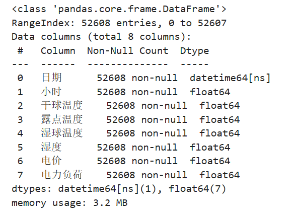
进一步统计缺失值
data_raw.isnull().sum()
2 构造训练数据
构造数据前先将数据变为数值类型
data_load = data_raw.iloc[:,2:].values构造训练数据,也是真正预测未来的关键。首先设置预测的timesteps时间步、predict_steps预测的步长(预测的步长应该比总的预测步长小),length总的预测步长,参数可以根据需要更改。
timesteps = 48*7 #构造x,为72个数据,表示每次用前72个数据作为一段
predict_steps = 6 #构造y,为12个数据,表示用后12个数据作为一段
length = 48 #预测多步,预测96个数据,每次预测96个,想想要怎么构造预测才能满足96?
feature_num = 6 #特征个数
通过前timesteps行历史数据预测后面predict_steps个数据,需要对数据集进行滚动划分(也就是前timesteps行的数据和后predict_steps行的数据训练,后面预测时就可通过timesteps行数据预测未来的predict_steps行数据)。这里需要注意的是,因为是多变量预测多变量,特征就是标签(例如,前5行[干球温度、露点温度、湿球温度、电价、电力负荷]预测第6行[干球温度、露点温度、湿球温度、电价、电力负荷],划分数据集时,就用前5行当做train_x,第6行作为train_y,此时的train_y有多列,而不是只有1列)。
# 构造数据集,用于真正预测未来数据
# 整体的思路也就是,前面通过前timesteps个数据训练后面的predict_steps个未来数据
# 预测时取出前timesteps个数据预测未来的predict_steps个未来数据。
def create_dataset(datasetx, datasety=None, timesteps=96*7, predict_size=12):datax = []  # 构造xdatay = []  # 构造yfor each in range(len(datasetx) - timesteps - predict_size):x = datasetx[each:each + timesteps]# 判断是否是单变量分解还是多变量分解if datasety is not None:y = datasety[each + timesteps:each + timesteps + predict_size]else:y = datasetx[each + timesteps:each + timesteps + predict_size]datax.append(x)datay.append(y)return datax, datay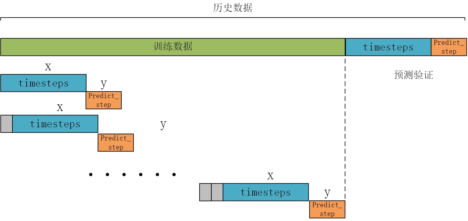
数据处理前,需要对数据进行归一化,按照上面的方法划分数据,这里返回划分的数据和归一化模型(变量和多变量的归一化不同,多变量归一化需要将X和Y分开归一化,不然会出现信息泄露的问题),此时的归一化相当于是单变量归一化,函数的定义如下:
# 数据归一化操作
def data_scaler(datax, datay=None, timesteps=36, predict_steps=6):# 数据归一化操作scaler1 = MinMaxScaler(feature_range=(0, 1))   datax = scaler1.fit_transform(datax)# 用前面的数据进行训练,留最后的数据进行预测# 判断是否是单变量分解还是多变量分解if datay is not None:scaler2 = MinMaxScaler(feature_range=(0, 1))datay = scaler2.fit_transform(datay)trainx, trainy = create_dataset(datax, datay, timesteps, predict_steps)trainx = np.array(trainx)trainy = np.array(trainy)return trainx, trainy, scaler1, scaler2else:trainx, trainy = create_dataset(datax, timesteps=timesteps, predict_size=predict_steps)trainx = np.array(trainx)trainy = np.array(trainy)return trainx, trainy, scaler1, None
然后分解的数据进行划分和归一化。通过前7天的48*7行数据预测后1天的数据48个,需要对数据集进行滚动划分(也就是前48*7行的数据和后6行的数据训练,后面预测时就可通过48*7行数据测未来的6行标签,然后将6行预测值添加到历史数据中,历史数据变为48*7+6个,再取出后48*7行数据进行预测,得到6行预测值,滚动进行预测直到预测完成,注意此时的预测值是行而不是个)
trainx, trainy, scalerx, scalery = data_scaler(data_load, timesteps=timesteps, predict_steps=predict_steps)
3 LSTM模型训练
首先划分训练集、测试集、验证数据:
train_x = trainx[:int(trainx.shape[0] * 0.8)]
train_y = trainy[:int(trainy.shape[0] * 0.8)]
test_x = trainx[int(trainx.shape[0] * 0.8):]
test_y = trainy[int(trainy.shape[0] * 0.8):]
test_x.shape, test_y.shape, train_x.shape, train_y.shape
首先搭建模型的常规操作,然后使用训练数据trainx和trainy进行训练,进行50个epochs的训练,每个batch包含64个样本(建议使用GPU进行训练)。
# 搭建LSTM训练函数
def LSTM_model_train(trainx, trainy, valx, valy, timesteps, predict_steps):# 调用GPU加速gpus = tf.config.experimental.list_physical_devices(device_type='GPU')for gpu in gpus:tf.config.experimental.set_memory_growth(gpu, True)# 搭建LSTM模型start_time = datetime.datetime.now()model = Sequential()model.add(LSTM(128, input_shape=(timesteps, trainx.shape[2]), return_sequences=True))model.add(BatchNormalization())  # 添加BatchNormalization层model.add(Dropout(0.2))model.add(LSTM(64, return_sequences=False))model.add(Dense(predict_steps * trainy.shape[2]))model.add(Reshape((predict_steps, trainy.shape[2])))# 使用自定义的Adam优化器opt = Adam(learning_rate=0.001)model.compile(loss="mean_squared_error", optimizer=opt)# 添加早停和模型保存的回调函数es = EarlyStopping(monitor='val_loss', mode='min', verbose=1, patience=10)mc = ModelCheckpoint('best_model.h5', monitor='val_loss', mode='min', save_best_only=True)# 训练模型,这里我假设你有一个验证集(valx, valy)history = model.fit(trainx, trainy, validation_data=(valx, valy), epochs=50, batch_size=64, callbacks=[es, mc])# 记录训练损失loss_history = history.history['loss']end_time = datetime.datetime.now()running_time = end_time - start_timereturn model, loss_history, running_time
然后进行训练,将训练的模型、损失和训练时间保存。
#模型训练
model, loss_history, running_time = LSTM_model_train(train_x, train_y, test_x, test_y, timesteps, predict_steps)
# 将模型保存为文件
model.save('lstm_model.h5')
训练损失可视化
plt.figure(dpi=100, figsize=(14, 5))
plt.plot(loss_history, markevery=5)
4 LSTM模型预测
4.1 分量预测
下面介绍文章中最重要,也是真正没有未来特征的情况下预测未来标签的方法。整体的思路也就是取出预测前48*7行数据预测未来的6行数据,然后见6行数据添加进历史数据,再预测6行数据,滚动预测。因为每次只能预测6行数据,但是我要预测48个数据,所以采用的就是循环预测的思路。每次预测的6行数据,添加到数据集中充当预测x,然后在预测新的6行y,再添加到预测x列表中,如此往复,最终预测出48行。(注意多变量预测多变量预测的是多列,预测单变量只有一列)
# #滚动predict
# #因为每次只能预测6个数据,但是我要预测6个数据,所以采用的就是循环预测的思路。
# #每次预测的6个数据,添加到数据集中充当预测x,然后在预测新的6个y,再添加到预测x列表中,如此往复,最终预测出48个点。
def predict_using_LSTM(model, data, timesteps, predict_steps, feature_num, length, scaler):predict_xlist = np.array(data).reshape(1, timesteps, feature_num) predict_y = np.array([]).reshape(0, feature_num)  # 初始化为空的二维数组print('predict_xlist', predict_xlist.shape)while len(predict_y) < length:# 从最新的predict_xlist取出timesteps个数据,预测新的predict_steps个数据predictx = predict_xlist[:,-timesteps:,:]# 变换格式,适应LSTM模型predictx = np.reshape(predictx, (1, timesteps, feature_num)) print('predictx.shape', predictx.shape)# 预测新值lstm_predict = model.predict(predictx)print('lstm_predict.shape', lstm_predict.shape)# 滚动预测# 将新预测出来的predict_steps个数据,加入predict_xlist列表,用于下次预测print('predict_xlist.shape', predict_xlist.shape)predict_xlist = np.concatenate((predict_xlist, lstm_predict), axis=1)print('predict_xlist.shape', predict_xlist.shape)# 预测的结果y,每次预测的6行数据,添加进去,直到预测length个为止lstm_predict = scaler.inverse_transform(lstm_predict.reshape(predict_steps, feature_num))predict_y = np.concatenate((predict_y, lstm_predict), axis=0)print('predict_y', predict_y.shape)return predict_y
然后对数据进行预测,得到预测结果。
from tensorflow.keras.models import load_model
model = load_model('best_model.h5')
pre_x = scalerx.fit_transform(data_load[-48*8:-48])
pre_y = data_load[-48:,-1]
y_predict = predict_using_LSTM(model, pre_x, timesteps, predict_steps, feature_num, length, scalerx)
4.2 可视化
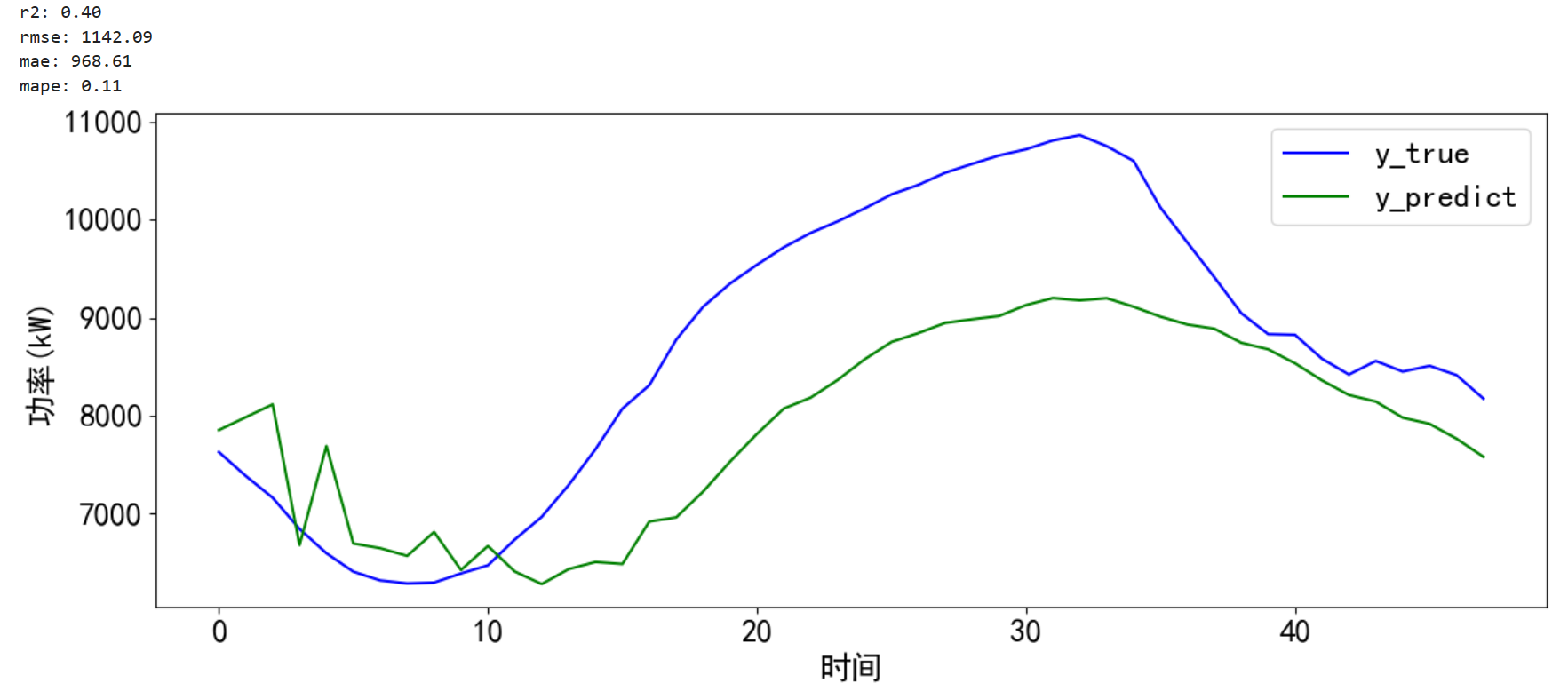
对预测的结果进行可视化并计算误差。
# 预测并计算误差和可视化
def error_and_plot(y_true,y_predict):# 计算误差r2 = r2_score(y_true, y_predict)rmse = mean_squared_error(y_true, y_predict, squared=False)mae = mean_absolute_error(y_true, y_predict)mape = mean_absolute_percentage_error(y_true, y_predict)print("r2: %.2f\nrmse: %.2f\nmae: %.2f\nmape: %.2f" % (r2, rmse, mae, mape))# 预测结果可视化cycol = cycle('bgrcmk')plt.figure(dpi=100, figsize=(14, 5))plt.plot(y_true, c=next(cycol), markevery=5)plt.plot(y_predict, c=next(cycol), markevery=5)plt.legend(['y_true', 'y_predict'])plt.xlabel('时间')plt.ylabel('功率(kW)')plt.show()   return 0
error_and_plot(pre_y, y_predict[:,-1])