- 🍨 本文为🔗365天深度学习训练营中的学习记录博客
- 🍖 原作者:K同学啊|接辅导、项目定制
1 前言
在计算机视觉领域,卷积神经网络(CNN)已经成为最主流的方法,比如GoogleNet,VGG-16,Incepetion等模型。CNN史上的一个里程碑事件是ResNet模型的出现,ResNet可以训练出更深的CNN模型,从而实现更高的准确率。ResNet模型的核心是通过建立前面层与后面层之间的“短路连接”(shortcut, skip connection),进而训练出更深的CNN网络。
DenseNet模型的基本思路与ResNet一致,但是它建立的是前面所有层与后面层的紧密连接(dense connection),它的名称也是由此而来。DenseNet的另一大特色是通过特征在channel上的的连接来实现特征重用(feature reuse)。这些特点让DenseNet在参数和计算成本更少的情形下实现比ResNet更优的性能,DenseNet也因此斩获CVPR2017的最佳论文奖。

其中DenseNet论文原文地址为:https://arxiv.org/pdf/1608.06993v5.pdf
2 设计理念
相比ResNet,DenseNet提出了一个更激进的密集连接机制:即互相连接所有的层,具体来说就是每个层都会接受前面所有层作为额外的输入。
图3为ResNet网络的残差连接机制,作为对比,图4为DenseNet的密集连接机制。可以看到,ResNet是每个层与前面的某层(一般是2~4层)短路连接在一起,连接方式是通过元素相加。而在DenseNet中,每个层都会与前面所有层在channel维度上链接(concat)在一起(即元素叠加),并作为下一层的输入。
对于一个L层的网络,DenseNet共包含个连接,相比ResNet,这是一种密集连接。而且DenseNet是直接concat来自不同层的特征图,这可以实现特征重用,提升效率,这一特点是DenseNet与ResNet最主要的区别。
2.1 标准神经网络

图2是一个标准的神经网络传播过程示意图,输入和输出的公式是,其中
是一个组合函数,通常包括BN、ReLu、Pooling、Conv等操作,
是第l层的输入的特征图(来自于l-1层的输出),
是第l层的输出的特征图。
2.2 ResNet
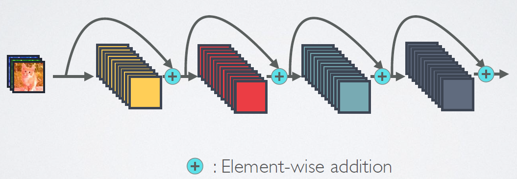
图3是ResNet的网络连接机制,由图可知是跨层相加,输入和输出的公式是
2.3 DenseNet
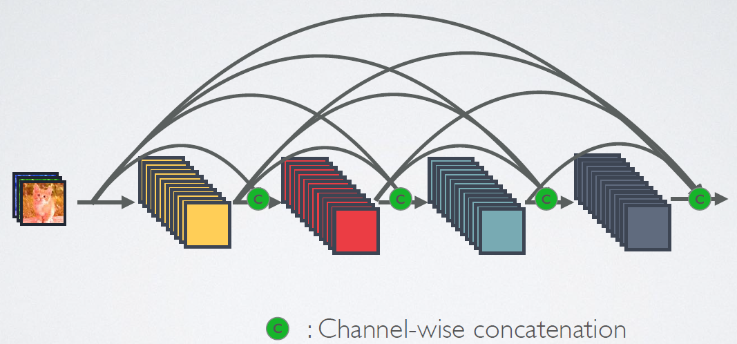
图4为DenseNet的连接机制,采用跨通道的concat的形式连接,会连接前面所有层作为输入,输入和输出的公式是。这里要注意所有层的输入都来源于前面所有层在channel维度的concat,以下动图形象表示这一操作。

3 网络结构
网络的具体实现细节如图6所示。
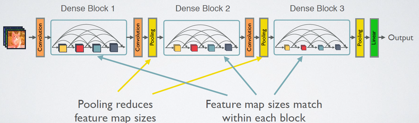
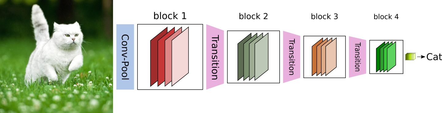
CNN网络一般要经过Pooling或者stride>1的Conv来降低特征图的大小,而DenseNet的密集连接方式需要特征图大小保持一致。为了解决这个问题,DenseNet网络中使用DenseBlock+Transition的结构,其中DenseBlock是包含很多层的模块,每个层的特征图大小相同,层与层之间采用密集连接方式。而Transition层是连接两个相邻的DenseBlock,并且通过Pooling使特征图大小降低。图7给出了DenseNet的网络结构,它共包含4个DenseBlock,各个DenseBlock之间通过Transition层连接在一起。
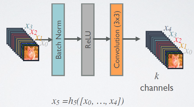
在DenseBlock中,各个层的特征图大小一致,可以在channel维度上连接。DenseBlock中的非线性组合函数的是BN+ReLU+3*3Conv的结构,如图8所示。另外,与ResNet不同,所有DenseBlock中各个层卷积之后均输出k个特征图,即得到的特征图的channel数为
,或者说采用k个卷积核。
在DenseNet称为growth rate,这是一个超参数。一般情况下使用较小的
(比如12),就可以得到较佳的性能。假定输入层的特征图的channel数为
,那么
层输入的channel数为
,因此随着层数的增加,尽管
设定的较小,DenseBlock的输入会非常多,不过这是由于特征重用所造成的,每个层仅有
个特征是自己独有的。
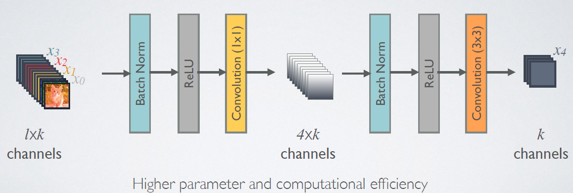
由于后面层的输入会非常大,DenseBlock内部采用bottleneck层来减少计算量,主要是原有的结构中增加1*1Conv,如图9所示,即BN+ReLU+1*1Conv+BN+ReLU+3*3Conv,称为DenseNet-B结构。其中1*1Conv得到个特征图,它起到的作用是降低特征数量,从而提升计算效率。
对于Trasition层,它主要是连接两个相邻的DenseBlock,并且降低特征图大小。Transition层包括一个1*1的卷积和2*2的AvgPooling,结构为BN+ReLU+1*1Conv+2*2AvgPooling。另外,Transition层可以起到压缩模型的作用。假定Transition层的上接DenseBlock得到特征图channels数为,Transition层可以产生
个特征(通过卷积层),其中
是压缩系数(compression rate)。当
时,特征个数经过Transition层没有变化,即无压缩,而当压缩系数小于1时,这种结构称为DenseNet-C,文中使用
。对于使用bootleneck层的DenseBlock结构和压缩系数小于1的Transition组合机构称为DenseNet-BC。
对于ImageNet数据集,图片输入大小为224*224,网络结构采用包含4个DenseBlock的DenseNet-BC,其首先是一个stride=2的7*7卷积层,然后是一个stride=2的3*3MaxPooling层,后面才进入DenseBlock。ImageNet数据集所采用的网络配置如表1所示:

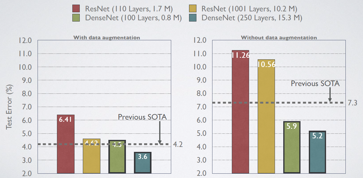
4 效果对比
5 使用Pytroch实现DenseNet121

图11为DenseNet121的具体网络结构,它与表1中的DenseNet121相对应。左边是整个DenseNet121的网络结构,其中粉色为DenseBlock,最右侧为其详细结构,灰色为Transition,中间为其详细结构。
5.1 前期工作
5.1.1 开发环境
电脑系统:ubuntu16.04
编译器:Jupter Lab
语言环境:Python 3.7
深度学习环境:pytorch
5.1.2 设置GPU
如果设备上支持GPU就使用GPU,否则注释掉这部分代码。
import torch
import torch.nn as nn
import torchvision.transforms as transforms
import torchvision
from torchvision import transforms, datasets
import os, PIL, pathlib, warningswarnings.filterwarnings("ignore")
device = torch.device("cuda" if torch.cuda.is_available() else "cpu")print(device)
5.1.3 导入数据
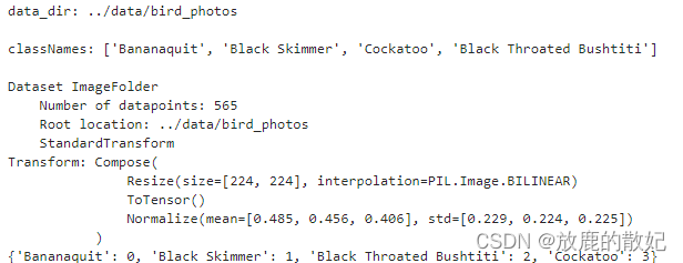
import os,PIL,random,pathlibdata_dir_str = '../data/bird_photos'
data_dir = pathlib.Path(data_dir_str)
print("data_dir:", data_dir, "\n")data_paths = list(data_dir.glob('*'))
classNames = [str(path).split('/')[-1] for path in data_paths]
print('classNames:', classNames , '\n')train_transforms = transforms.Compose([transforms.Resize([224, 224]),  # resize输入图片transforms.ToTensor(),  # 将PIL Image或numpy.ndarray转换成tensortransforms.Normalize(mean=[0.485, 0.456, 0.406],std=[0.229, 0.224, 0.225])  # 从数据集中随机抽样计算得到
])total_data = datasets.ImageFolder(data_dir_str, transform=train_transforms)
print(total_data)
print(total_data.class_to_idx)
结果输出如图:
5.1.4 划分数据集
train_size = int(0.8 * len(total_data))
test_size = len(total_data) - train_size
train_dataset, test_dataset = torch.utils.data.random_split(total_data, [train_size, test_size])
print(train_dataset, test_dataset)batch_size = 4
train_dl = torch.utils.data.DataLoader(train_dataset, batch_size=batch_size,shuffle=True,num_workers=1,pin_memory=False)
test_dl = torch.utils.data.DataLoader(test_dataset, batch_size=batch_size,shuffle=True,num_workers=1,pin_memory=False)for X, y in test_dl:print("Shape of X [N, C, H, W]:", X.shape)print("Shape of y:", y.shape, y.dtype)break
结果输出如图:
5.2 搭建DenseNet121
5.2.1 DenseBlock中的Bottleneck
import torch
from torch import nnclass _DenseLayer(nn.Sequential):"""DenseBlock的基本单元(使用bottleneck)"""def __init__(self, num_input_features, growth_rate, bn_size, drop_rate):super(_DenseLayer, self).__init__()self.add_module("norm1", nn.BatchNorm2d(num_input_features))self.add_module("relu1", nn.ReLU(inplace=True))self.add_module("conv1", nn.Conv2d(num_input_features, bn_size*growth_rate,kernel_size=1, stride=1, bias=False))self.add_module("norm2", nn.BatchNorm2d(bn_size*growth_rate))self.add_module("relu2", nn.ReLU(inplace=True))self.add_module("conv2", nn.Conv2d(bn_size*growth_rate, growth_rate,kernel_size=3, stride=1, padding=1, bias=False))self.drop_rate = drop_ratedef forward(self, x):new_features = super(_DenseLayer, self).forward(x)if self.drop_rate > 0:new_features = F.dropout(new_features, p=self.drop_rate, training=self.training)return torch.cat([x, new_features], 1)
5.2.2 DenseBlock层
class _DenseBlock(nn.Sequential):def __init__(self, num_layer, num_input_features, bn_size, growth_rate, drop_rate):super(_DenseBlock, self).__init__()for i in range(num_layer):layer = _DenseLayer(num_input_features+i*growth_rate, growth_rate, bn_size, drop_rate)self.add_module("denselayer%d" % (i+1,), layer)5.2.3 Transition层
class _Transition(nn.Sequential):def __init__(self, num_input_features, num_output_features):super(_Transition, self).__init__()self.add_module("norm", nn.BatchNorm2d(num_input_features))self.add_module("relu", nn.ReLU(inplace=True))self.add_module("conv", nn.Conv2d(num_input_features, num_output_features,kernel_size=1, stride=1, bias=False))self.add_module("pool", nn.AvgPool2d(2, stride=2)) 5.2.4 DenseNet-BC
import torch.nn.functional as F#from collections import OrderedDict
import collectionstry:from collections import OrderedDict
except ImportError:OrderedDict = dictclass DenseNet(nn.Module):"DenseNet-BC model"def __init__(self, growth_rate=32, block_config=(6, 12, 24, 16), num_init_features=64,bn_size=4, compression_rate=0.5, drop_rate=0, num_classes=4):"""growth_rate:(int) number of filters used in DenseLayer, 'k' in the paperblock_config:(list of 4 ints) number of layers in each DenseBlocknum_init_features:(int) number of filters in the first Conv2dbn_size:(int) the factor using in the bottleneck layercompression_rate:(float) the compression rate used in Trasition Layerdrop_rate:(float) the drop rate after each DenseLayernum_classes:(int) number of classes for classification"""super(DenseNet, self).__init__()# first Conv2dself.features = nn.Sequential(OrderedDict([("conv0", nn.Conv2d(3, num_init_features, kernel_size=7, stride=2, padding=3, bias=False)),("norm0", nn.BatchNorm2d(num_init_features)),("relu0", nn.ReLU(inplace=True)),("pool0", nn.MaxPool2d(3, stride=2, padding=1))]))# DenseBlocknum_features = num_init_featuresfor i,num_layers in enumerate(block_config):block = _DenseBlock(num_layers, num_features, bn_size, growth_rate, drop_rate)self.features.add_module("denseblock%d" % (i + 1), block)num_features += num_layers*growth_rateif i != len(block_config) - 1:transition = _Transition(num_features, int(num_features*compression_rate))self.features.add_module("transition%d" % (i+1), transition)num_features = int(num_features * compression_rate)# final bn+reluself.features.add_module("norm5", nn.BatchNorm2d(num_features))self.features.add_module("relu5", nn.ReLU(inplace=True))# classification layerself.classifier = nn.Linear(num_features, num_classes)# params initializationfor m in self.modules():if isinstance(m, nn.Conv2d):nn.init.kaiming_normal_(m.weight)elif isinstance(m, nn.BatchNorm2d):nn.init.constant_(m.bias, 0)nn.init.constant_(m.weight, 1)elif isinstance(m, nn.Linear):nn.init.constant_(m.bias, 0)def forward(self, x):features = self.features(x)out = F.avg_pool2d(features, 7, stride=1).view(features.size(0), -1)out = self.classifier(out)return out
5.2.5 DenseNet121
import redef densenet121(pretrained=False, **kwargs):# DenseNet121model = DenseNet(num_init_features=64, growth_rate=32, block_config=(6,12,24,16), ** kwargs)if pretrained:# '.' are no longer in module names, but pervious _DenseLayer# has keys 'norm.1','relu.1','conv.1','norm.2','relu.2','conv.2'.# They are also in the checkpoints in model_urls.This pattern is used# to find find such keys.pattern = re.compile(r'^(.*denselayer\d+\.(?:norm|relu\conv))\.((?:[12])\.(?:weight|bias|running_mean|running_var))$')state_dir = model_zoo.load_url(model_urls['densenet121'])for key in list(state_dict.key()):res = pattern.match(key)if res:new_key = res.group(1) + res.group(2)state_dict[new_key] = state_dict[key]del state_dict[key]model.load_state_dict(state_dict)return modelmodel = densenet121().to(device)
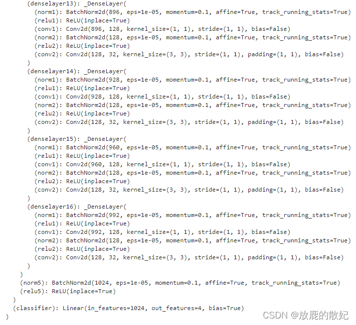
model结果输出如下(由于结果太长,只展示最前面和最后面):

(中间省略)
5.2.6 查看模型详情
# 统计模型参数量以及其他指标
import torchsummary as summary
summary.summary(model, (3, 224, 224))
结果输出如下(由于结果太长,只展示最前面和最后面):
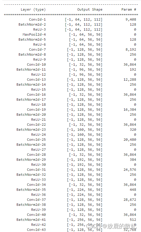
(中间省略)

5.3 训练模型
5.3.1 编写训练函数
# 训练循环
def train(dataloader, model, loss_fn, optimizer):size = len(dataloader.dataset)  # 训练集的大小num_batches = len(dataloader)   # 批次数目, (size/batch_size,向上取整)train_loss, train_acc = 0, 0  # 初始化训练损失和正确率for X, y in dataloader:  # 获取图片及其标签X, y = X.to(device), y.to(device)# 计算预测误差pred = model(X)          # 网络输出loss = loss_fn(pred, y)  # 计算网络输出pred和真实值y之间的差距,y为真实值,计算二者差值即为损失# 反向传播optimizer.zero_grad()  # grad属性归零loss.backward()        # 反向传播optimizer.step()       # 每一步自动更新# 记录acc与losstrain_acc  += (pred.argmax(1) == y).type(torch.float).sum().item()train_loss += loss.item()train_acc  /= sizetrain_loss /= num_batchesreturn train_acc, train_loss
5.3.2 编写测试函数
def test(dataloader, model, loss_fn):size = len(dataloader.dataset) # 训练集的大小num_batches = len(dataloader) # 批次数目, (size/batch_size,向上取整)test_loss, test_acc = 0, 0 # 初始化测试损失和正确率# 当不进行训练时,停止梯度更新,节省计算内存消耗# with torch.no_grad():for imgs, target in dataloader: # 获取图片及其标签with torch.no_grad():imgs, target = imgs.to(device), target.to(device)# 计算误差tartget_pred = model(imgs) # 网络输出loss = loss_fn(tartget_pred, target) # 计算网络输出和真实值之间的差距,targets为真实值,计算二者差值即为损失# 记录acc与losstest_loss += loss.item()test_acc += (tartget_pred.argmax(1) == target).type(torch.float).sum().item()test_acc /= sizetest_loss /= num_batchesreturn test_acc, test_loss5.3.3 正式训练
import copyoptimizer = torch.optim.Adam(model.parameters(), lr = 1e-4)
loss_fn = nn.CrossEntropyLoss() #创建损失函数epochs = 40train_loss = []
train_acc = []
test_loss = []
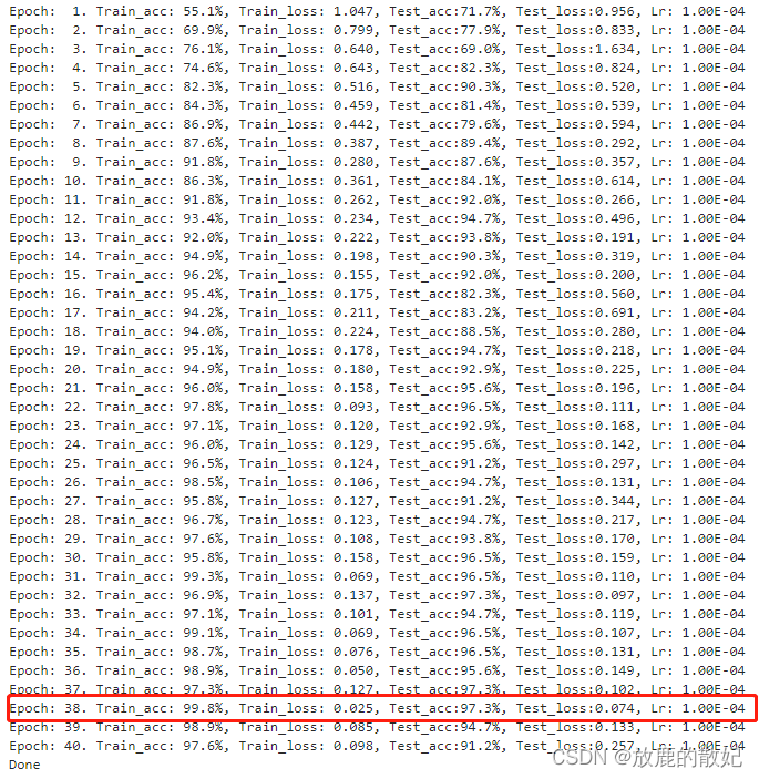
test_acc = []best_acc = 0 #设置一个最佳准确率,作为最佳模型的判别指标if hasattr(torch.cuda, 'empty_cache'):torch.cuda.empty_cache()for epoch in range(epochs):model.train()epoch_train_acc, epoch_train_loss = train(train_dl, model, loss_fn, optimizer)#scheduler.step() #更新学习率(调用官方动态学习率接口时使用)model.eval()epoch_test_acc, epoch_test_loss = test(test_dl, model, loss_fn)#保存最佳模型到best_modelif epoch_test_acc > best_acc:best_acc = epoch_test_accbest_model = copy.deepcopy(model)train_acc.append(epoch_train_acc)train_loss.append(epoch_train_loss)test_acc.append(epoch_test_acc)test_loss.append(epoch_test_loss)#获取当前的学习率lr = optimizer.state_dict()['param_groups'][0]['lr']template = ('Epoch: {:2d}. Train_acc: {:.1f}%, Train_loss: {:.3f}, Test_acc:{:.1f}%, Test_loss:{:.3f}, Lr: {:.2E}')print(template.format(epoch+1, epoch_train_acc*100, epoch_train_loss, epoch_test_acc*100, epoch_test_loss, lr))PATH = './J3_best_model.pth'
torch.save(model.state_dict(), PATH)print('Done')结果输出如下:
5.4 结果可视化
import matplotlib.pyplot as plt
#隐藏警告
import warnings
warnings.filterwarnings("ignore") #忽略警告信息
plt.rcParams['font.sans-serif'] = ['SimHei'] # 用来正常显示中文标签
plt.rcParams['axes.unicode_minus'] = False # 用来正常显示负号
plt.rcParams['figure.dpi'] = 100 #分辨率epochs_range = range(epochs)plt.figure(figsize=(12, 3))
plt.subplot(1, 2, 1)plt.plot(epochs_range, train_acc, label='Training Accuracy')
plt.plot(epochs_range, test_acc, label='Test Accuracy')
plt.legend(loc='lower right')
plt.title('Training and Validation Accuracy')plt.subplot(1, 2, 2)
plt.plot(epochs_range, train_loss, label='Training Loss')
plt.plot(epochs_range, test_loss, label='Test Loss')
plt.legend(loc='upper right')
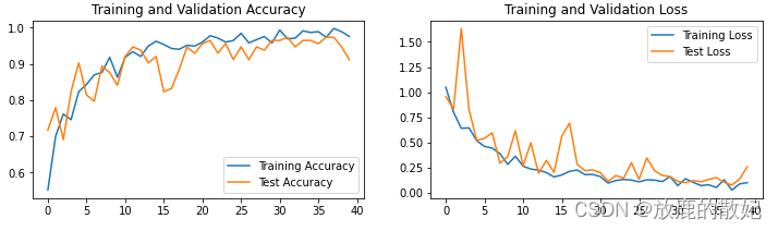
plt.title('Training and Validation Loss')
plt.show()结果输出如下:
6 使用Tensorflow实现DenseNet121
6.1 前期工作
6.1.1 开发环境
电脑系统:ubuntu16.04
编译器:Jupter Lab
语言环境:Python 3.7
深度学习环境:tensorflow
6.1.2 设置GPU
如果设备上支持GPU就使用GPU,否则注释掉这部分代码。
import tensorflow as tfgpus = tf.config.list_physical_devices("GPU")if gpus:tf.config.experimental.set_memory_growth(gpus[0], True) # 设置GPU显存用量按需使用tf.config.set_visible_devices([gpus[0]], "GPU")6.1.2 导入数据
import matplotlib.pyplot as plt
# 支持中文
plt.rcParams['font.sans-serif'] = ['SimHei'] # 用来正常显示中文标签
plt.rcParams['axes.unicode_minus'] = False # 用来正常显示负号import os, PIL, pathlib
import numpy as npfrom tensorflow import keras
from tensorflow.keras import layers,modelsdata_dir = "../data/bird_photos"
data_dir = pathlib.Path(data_dir)image_count = len(list(data_dir.glob('*/*')))
print("图片总数为:", image_count)
6.1.3 加载数据
batch_size = 8
img_height = 224
img_width = 224train_ds = tf.keras.preprocessing.image_dataset_from_directory(data_dir,validation_split=0.2,subset="training",seed=123,image_size=(img_height, img_width),batch_size=batch_size)val_ds = tf.keras.preprocessing.image_dataset_from_directory(data_dir,validation_split=0.2,subset="validation",seed=123,image_size=(img_height, img_width),batch_size=batch_size)class_Names = train_ds.class_names
print("class_Names:",class_Names)
输出结果如下:

6.1.4 可视化数据
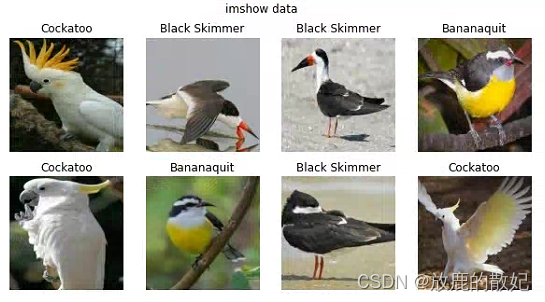
plt.figure(figsize=(10, 5)) # 图形的宽为10,高为5
plt.suptitle("imshow data")for images,labels in train_ds.take(1):for i in range(8):ax = plt.subplot(2, 4, i+1)plt.imshow(images[i].numpy().astype("uint8"))plt.title(class_Names[labels[i]])plt.axis("off")
输出结果如下:
6.1.5 检查数据
for image_batch, lables_batch in train_ds:print(image_batch.shape)print(lables_batch.shape)break输出结果如下:
![]()
6.1.6 配置数据集
AUTOTUNE = tf.data.AUTOTUNEtrain_ds = train_ds.cache().shuffle(1000).prefetch(buffer_size=AUTOTUNE)
val_ds = val_ds.cache().prefetch(buffer_size=AUTOTUNE)
6.2 搭建DenseNet121
6.2.1 DenseNet121
import tensorflow as tf
import tensorflow.keras.layers as layers
from tensorflow.keras import regularizers
# from tensorflow.keras.models import Modelfrom tensorflow.keras.layers import Input,Activation,BatchNormalization,Flatten
from tensorflow.keras.layers import Dense,Conv2D,MaxPooling2D,ZeroPadding2D,AveragePooling2D
from tensorflow.keras.models import Modeldef regularized_padded_conv2d(*args, **kwargs):"""带标准化的卷积"""return layers.Conv2D(*args, **kwargs,padding='same', kernel_regularizer=regularizers.l2(5e-5), bias_regularizer=regularizers.l2(5e-5),kernel_initializer='glorot_normal')def DenseLayer(x, growth_rate, bn_size, drop_rate, layerName):new_features = layers.BatchNormalization(name=layerName+"_norm1")(x)new_features = layers.Activation('relu', name=layerName+"_relu1")(new_features)new_features = regularized_padded_conv2d(filters=bn_size*growth_rate, kernel_size=1, strides=1, use_bias=False, name=layerName+"_conv1")(new_features)new_features = layers.BatchNormalization(name=layerName+"_norm2")(new_features)new_features = layers.Activation('relu', name=layerName+"_relu2")(new_features)new_features = regularized_padded_conv2d(filters=growth_rate, kernel_size=3, strides=1, use_bias=False, name=layerName+"_conv2")(new_features)if drop_rate > 0:new_features = layers.Dropout(rate=drop_rate)(new_features)return layers.concatenate([x, new_features], axis=-1)def DenseBlock(x, num_layer, bn_size, growth_rate, drop_rate, blockName):for i in range(num_layer):x = DenseLayer(x, growth_rate=growth_rate, bn_size=bn_size, drop_rate=drop_rate, layerName=blockName+'_'+str(i+1))return xdef Transition(x, num_output_features, blockName):x = layers.BatchNormalization(name=blockName+"_norm")(x)x =  layers.Activation('relu', name=blockName+"_relu")(x)x = regularized_padded_conv2d(filters=num_output_features, kernel_size=1, strides=1, use_bias=False, name=blockName+"_conv")(x)x = layers.AveragePooling2D(pool_size=2, strides=2, padding='same', name=blockName+'_pool')(x)return xdef densenet121(input_shape=[224,224,3], growth_rate=32, block_config=(6, 12, 24, 16), num_init_features=64,bn_size=4, compression_rate=0.5, drop_rate=0, num_classes=4, classifier_activation='softmax'):img_input = Input(shape=input_shape)# first Conv2dx = regularized_padded_conv2d(filters=num_init_features, kernel_size=7, strides=2, use_bias=False, name="pre_conv")(img_input)x = layers.BatchNormalization(name="pre_norm")(x)x = layers.Activation('relu', name="pre_relu")(x)x = layers.MaxPool2D(pool_size=3, strides=2, padding='same')(x)# DenseBlocknum_features = num_init_featuresfor i,num_layer in enumerate(block_config):x = DenseBlock(x, num_layer=num_layer, bn_size=bn_size, growth_rate=growth_rate, drop_rate=drop_rate, blockName="DenseBlock_"+str(i+1))num_features += num_layer*growth_rateif i != len(block_config) - 1:num_features = int(num_features * compression_rate)x = Transition(x, num_output_features=num_features, blockName="TransBlock_"+ str(i+1))# final bn+relux = layers.BatchNormalization(name="norm5")(x)x = layers.Activation('relu', name="relu5")(x)x = layers.AveragePooling2D(pool_size=7, strides=1, name='pool5')(x) #GlobalAveragePooling2D# classification layerx = Dense(num_classes, activation=classifier_activation, name='classifier')(x)model = Model(img_input, x, name='densenet121')# # 加载预训练模型# model.load_weights("resnet50_weights_tf_dim_ordering_tf_kernels.h5")return model
6.2.2 查看模型详情
model = densenet121()
model.summary()
结果如图所示(由于内容较长,只截取前后部分内容):

(中间部分省略)

6.3 训练模型
# 设置优化器
opt = tf.keras.optimizers.Adam(learning_rate=1e-6)
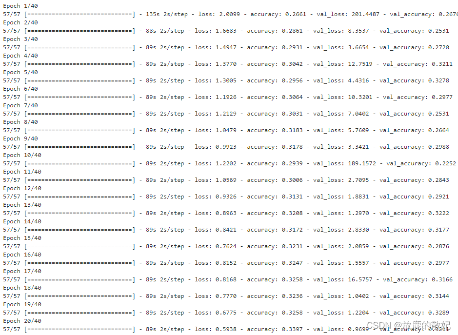
model.compile(optimizer="adam",loss='sparse_categorical_crossentropy',metrics=['accuracy'])epochs = 40
history = model.fit(train_ds,validation_data=val_ds,epochs=epochs)结果如下图所示:

6.4 模型评估
acc = history.history['accuracy']
val_acc = history.history['val_accuracy']loss = history.history['loss']
val_loss = history.history['val_loss']epochs_range = range(epochs)plt.figure(figsize=(12, 4))
plt.subplot(1, 2, 1)
plt.suptitle("DenseNet test")plt.plot(epochs_range, acc, label='Training Accuracy')
plt.plot(epochs_range, val_acc, label='Validation Accuracy')
plt.legend(loc='lower right')
plt.title('Training and Validation Accuracy')plt.subplot(1, 2, 2)
plt.plot(epochs_range, loss, label='Training Loss')
plt.plot(epochs_range, val_loss, label='Validation loss')
plt.legend(loc='upper right')
plt.title('Training and Validation loss')
plt.show()
结果如下图所示:

结合训练时的输出结果和模型评估图可以看出,训练的效果不理想,修改了learing_rate效果也不明显,后续继续尝试和分析。