弹性波动力学笔记(十)罗格里德斯公式推导

Note: Derivation of the Rodriguez Formula

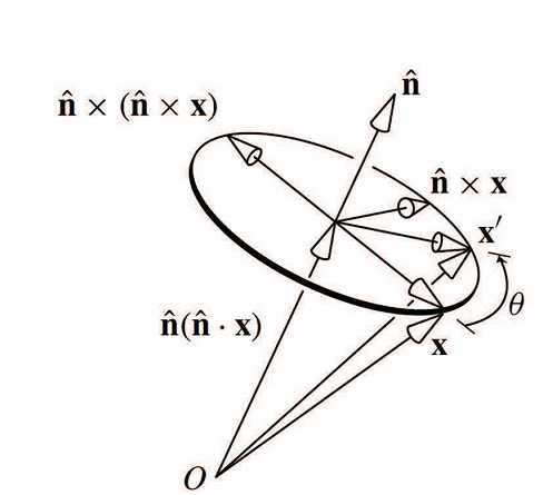
In this Note, we will derive a formula for \(\mathbf{R}(\widehat{\mathbf{n}},\theta)\) . Consider the three dimensional rotation of a vector \(\boldsymbol{x}\) into a vector \(\boldsymbol{x^{'}}\), which is described algebraically by the equation,

\[\boldsymbol{x^{'}}=\mathbf{R}(\widehat{\mathbf{n}},\theta)\boldsymbol{x},\space where\space ||\boldsymbol{x^{'}}||=||\boldsymbol{x}|| \tag{1} \]

Since we are rotating the vector \(\boldsymbol{x}\) around an axis that is parallel to the unit vector \(\widehat{\boldsymbol{n}}\) , it is convenient to decompose \(\boldsymbol{x}\) into a component parallel to the unit vector \(\widehat{\boldsymbol{n}}\) and a component perpendicular to \(\boldsymbol{n}\). Such a decomposition has the following form,

\[\boldsymbol{x}=\boldsymbol{x}_{\perp}+\boldsymbol{x}_{\|} \space where \space \boldsymbol{x}_{\|}=x_{\|}\widehat{\boldsymbol{n}} \tag{2} \]

Note that \(\boldsymbol{x}_{\perp}\) is vector that lives in the three-dimensional plane perpendicular to \(\widehat{\boldsymbol{n}}\) ,whereas \(\boldsymbol{x}_{\|}\) lives one dimensional line parallel to \(\widehat{\boldsymbol{n}}\) . In the above notation, the unbolded symbol \(x_{\|}\) is the length of the vector \(\boldsymbol{x}_{\|}\).

One can obtain convenient formula for \(\boldsymbol{x}_{\|}\) and \(\boldsymbol{x}_{\perp}\) in terms of \(\boldsymbol{x}\) and \(\widehat{\boldsymbol{n}}\) as follows. First, note that

\[\widehat{\boldsymbol{n}}\cdot\boldsymbol{x}_{\perp}=0,\space \widehat{\boldsymbol{n}}\times\boldsymbol{x}_{\|}=0\tag{3} \]

which is equivalent to the statements that \(\boldsymbol{x}_{\perp}\) is perpendicular to \(\widehat{\mathbf{n}}\) and \(\boldsymbol{x}_{\|}\) is parallel to \(\widehat{\boldsymbol{n}}\) . If we now compute the dot product \(\widehat{\boldsymbol{n}} \cdot \boldsymbol{x}\) using equations (1) and (2), then it follows that

\[\widehat{\boldsymbol{n}}\cdot\boldsymbol{x}=\widehat{\boldsymbol{n}}\cdot\boldsymbol{x}_{\|}=x_{\|} \tag{4} \]

Substituting for \(x_{\|}\) back in equation(2) yields,

\[\boldsymbol{x}_{\|}=\widehat{\boldsymbol{n}}(\widehat{\boldsymbol{n}}\cdot\boldsymbol{x})\tag{5} \]

From this result, we can derive an equation for \(\boldsymbol{x}_{\perp}\). Using equation (2) and (5) ,

\[\boldsymbol{x}_{\perp}=\boldsymbol{x}-\boldsymbol{x}_{\|}=\boldsymbol{x}-\widehat{\boldsymbol{n}}(\widehat{\boldsymbol{n}}\cdot\boldsymbol{x})\tag{6} \]

We can rewrite the above equation in a fancier way by using a well know vector identity, which yields

\[\widehat{\boldsymbol{n}}\times(\widehat{\boldsymbol{n}}\times\boldsymbol{x})=\widehat{\boldsymbol{n}}(\widehat{\boldsymbol{n}}\cdot\boldsymbol{x})-\boldsymbol{x}\tag{7} \]

Hence, an equivalent form of equation(7) is

\[\boldsymbol{x}_{\perp}=-\widehat{\boldsymbol{n}}\times(\widehat{\boldsymbol{n}}\times\boldsymbol{x}) \tag{8} \]

To derive a formula for \(\boldsymbol{x}^{\prime}=\mathbf{R}(\widehat{\boldsymbol{n}},\theta)\boldsymbol{x}\) ,the key observation is the following. By decomposing \(\boldsymbol{x}\) according to equation (1), a rotation about an axis that points in the \(\widehat{\boldsymbol{n}}\) direction only rotates \(\boldsymbol{x}_{\perp}\), while leaving \(\boldsymbol{x}_{\|}\) unchanged. Since \(\boldsymbol{x}_{\perp}\) lives a plane, all we need to perform a two-dimensional rotation of \(\boldsymbol{x}_{\perp}\). The end result is the rotated vector,

\[\boldsymbol{x}^{\prime}=\boldsymbol{x}^{\prime}_{\|}+\boldsymbol{x}^{\prime}_{\perp} \tag{9} \]

where \(\boldsymbol{x}_{\perp}=\mathbf{R}(\widehat{\boldsymbol{n}},\theta)\boldsymbol{x}_{\perp}\),\(\boldsymbol{x}_{\|}=\mathbf{R}(\widehat{\boldsymbol{n}},\theta)\boldsymbol{x}_{\|}=\boldsymbol{x}_{\|}\).

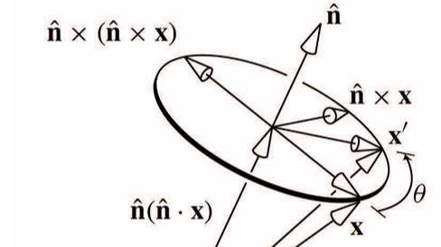
Referring to Figure 1 and 2, we see that the rotated vector \(\boldsymbol{x^{\prime}}_{\perp}\) by an angle \(\theta\) in the two dimensional \(x-y\) plane. In order to check that Figure 2 makes sense as drawn, one should verify that \(\boldsymbol{x}_{\perp}\) is perpendicular to \(\widehat{\boldsymbol{n}}\times{\boldsymbol{x}}\),and both these vectors are mutually perpendicular to the unit vector \(\widehat{\mathbf{n}}\) . Moreover,\(\|\boldsymbol{x}_{\perp}\|=\|\widehat{\boldsymbol{n}}\times\boldsymbol{x}\|\) as indicated in Figure 2.

Figure2

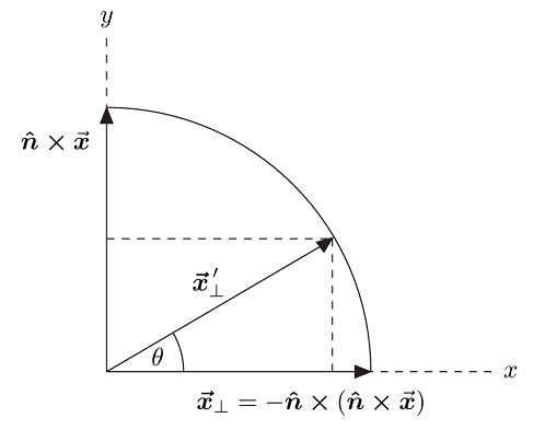
It is convenient to define the following two unit vectors that point along \(x\) and \(y\) axes, respectively,

\[\begin{equation} \begin{aligned} \boldsymbol{\widehat{e}}_1&=\frac{\boldsymbol{x}_{\perp}}{\|\boldsymbol{x}_{\perp}\|}=\frac{-\boldsymbol{\widehat{n}}\times(\boldsymbol{\widehat{n}}\times\boldsymbol{x})}{\|\boldsymbol{\widehat{n}}\times(\boldsymbol{\widehat{n}}\times\boldsymbol{x})\|}\\ \boldsymbol{\widehat{e}}_2&=\frac{\boldsymbol{\widehat{n}}\times\boldsymbol{x}}{\|\boldsymbol{\widehat{n}}\times\boldsymbol{x}\|} \end{aligned} \tag{11} \end{equation} \]

Note that \(\boldsymbol{\widehat{n}}\cdot\boldsymbol{\widehat{e}}_1=\boldsymbol{\widehat{n}}\cdot\boldsymbol{\widehat{e}}_2=0\), since for any vector \(\boldsymbol{a}\) the cross product \(\boldsymbol{\widehat{n}}\times\boldsymbol{a}\) is perpendicular to \(\boldsymbol{\widehat{n}}\) by the definition of the cross product. Thus, \(\boldsymbol{\widehat{e}}_1\)and\(\boldsymbol{\widehat{e}}_2\) lie in the plane perpendicular to \(\boldsymbol{\widehat{n}}\) as required. To show that \(\boldsymbol{\widehat{e}}_1\)and\(\boldsymbol{\widehat{e}}_2\) are orthogonal, we can use equation(7),

\[[\widehat{\boldsymbol{n}}(\widehat{\boldsymbol{n}}\cdot\boldsymbol{x})-\boldsymbol{x}]\cdot(\boldsymbol{\widehat{n}}\times\boldsymbol{x})=\widehat{\boldsymbol{n}}(\widehat{\boldsymbol{n}}\cdot\boldsymbol{x})\cdot(\boldsymbol{\widehat{n}}\times\boldsymbol{x})-\boldsymbol{x}\cdot(\boldsymbol{\widehat{n}}\times\boldsymbol{x})=0 \tag{12} \]

where again we have noted that \(\boldsymbol{\widehat{n}}\times\boldsymbol{x}\) is perpendicular both to \(\boldsymbol{\widehat{n}}\) and to \(\boldsymbol{x}\). Finally, in order to verify that \(\|\boldsymbol{x}_{\perp}\|=\|\boldsymbol{\widehat{n}}\times\boldsymbol{x}\|\), we shall employ the well known vector identity, \(\|a\times b\|=\|a\|^2\|b\|^2-(a\cdot b)^2\). It then follows that

\[\|\boldsymbol{x}_{\perp}\|^2=\|\widehat{\boldsymbol{n}}\times(\widehat{\boldsymbol{n}}\times\boldsymbol{x})\|^2=\|\boldsymbol{\widehat{n}}\times\boldsymbol{x}\|^2=\|\boldsymbol{x}\|^2-(\boldsymbol{\widehat{n}}\cdot \boldsymbol{x})^2 \tag{13} \]

Figure 2 provides a geometric method for finding an expression for \(\boldsymbol{x^{\prime}}_{\perp}\) down to the \(x\) and \(y\) axes in Figure 2,it follows that \(\boldsymbol{x^{\prime}}_{\perp}\) is the vector sum of the two projected vectors. That is,

\[\boldsymbol{x^{\prime}}_{\perp}=(\boldsymbol{\widehat{n}}\times\boldsymbol{x})\sin{\theta}-[\widehat{\boldsymbol{n}}\times(\widehat{\boldsymbol{n}}\times\boldsymbol{x})]\cos{\theta} \tag{14} \]

It is straightforward to verify that \(\|\boldsymbol{x}^{\prime}_{\perp}\|=\|\boldsymbol{x}_{\perp}\|\), which implies that a counterclockwise rotation of \(\boldsymbol{x}_{\perp}\) by an angle \(\theta\) yields \(\boldsymbol{x^{\prime}}_{\perp}\), as required. In particular, in light of equations (12) and (13) one can compute \(\|\boldsymbol{x}^{\prime}\|^2=\boldsymbol{x}^{\prime}\cdot\boldsymbol{x}^{\prime}\) as follows:

\[\|\boldsymbol{x^{\prime}}_{\perp}\|^2=\|\boldsymbol{\widehat{n}}\times\boldsymbol{x}\|^2\sin^2{\theta}+\|\widehat{\boldsymbol{n}}\times(\widehat{\boldsymbol{n}}\times\boldsymbol{x})\|\cos^2{\theta}=\|\boldsymbol{x}_{\perp}\|^2(\sin^2{\theta}+\cos^2{\theta})=\|\boldsymbol{x}_{\perp}\| \tag{15} \]

Finally, by using equation (5)

\[\boldsymbol{x^{\prime}}_{\|}=\boldsymbol{x}_{\|}=\boldsymbol{\widehat{n}}(\boldsymbol{\widehat{n}}\cdot\boldsymbol{x}) \tag{16} \]

since \(\boldsymbol{x}_{\perp}\) lies along the direction of the axis rotation, \(\boldsymbol{\widehat{n}}\) ,and thus does not rotate. Adding the results of equation (14) and (16), we conclude that

\[\boldsymbol{x^{\prime}}=\boldsymbol{x^{\prime}}_{\|}+\boldsymbol{x^{\prime}}_{\perp}=\boldsymbol{\widehat{n}}(\boldsymbol{\widehat{n}}\cdot\boldsymbol{x})+(\boldsymbol{\widehat{n}}\times\boldsymbol{x})\sin{\theta}-[\widehat{\boldsymbol{n}}\times(\widehat{\boldsymbol{n}}\times\boldsymbol{x})]\cos{\theta} \tag{17} \]

Equation 17 is equivalent to the equation \(\boldsymbol{x^{\prime}}=\mathbf{R}(\boldsymbol{\widehat{n}},\theta)\boldsymbol{x}\), where the matrix \(\mathbf{R}(\boldsymbol{\widehat{n}},\theta)\) is axes rotation matrix. To verify this assertion is a straightforward but tedious exercise in expanding out the components of the corresponding cross products. However, if you are comfortable in using the Levi-Civita epsilon symbol, then one can directly obtain the Rodriguez formula by writing equation (17) in terms of components. The components of the cross product are given by

\[(\boldsymbol{\widehat{n}}\times\boldsymbol{x})_i=-(\boldsymbol{x}\times\boldsymbol{\widehat{n}})_i=-\sum_{j=1}^3\sum_{k=1}^3\epsilon_{ijk}x_jn_k\tag{18} \]

Similarly,using equation (8)

\[[\boldsymbol{\widehat{n}}\times(\boldsymbol{\widehat{n}}\times{\boldsymbol{x}})]_i=[\boldsymbol{\widehat{n}}(\boldsymbol{\widehat{n}}\cdot\boldsymbol{x})-\boldsymbol{x}]_i=n_i\left(\sum_{j=1}^3n_jx_j\right)-x_i \tag{19} \]

Hence, the components of equation (17)

\[\begin{equation} \begin{aligned} x^{\prime}_i&=n_i\left(\sum_{j=1}^3n_jx_j\right)-\sin{\theta}\sum_{j=1}^3\sum_{k=1}^3\epsilon_{ijk}x_jn_k-\cos{\theta}\left[n_i\left(\sum_{j=1}^3n_jx_j\right)-x_i\right]\\ &=x_i\cos{\theta}+\sum_{j=1}^3\left[(1-\cos{\theta})n_in_j-\sin{\theta}\sum_{k=1}^3\epsilon_{ijk}n_k\right]x_j\\ &=\delta_{ij}x_j\cos{\theta}+\sum_{j=1}^3\left[(1-\cos{\theta})n_in_j-\sin{\theta}\sum_{k=1}^3\epsilon_{ijk}n_k\right]x_j\\ &=\sum_{j=1}^3\left[\delta_{ij}\cos{\theta}+(1-\cos{\theta})n_in_j-\sin{\theta}\sum_{k=1}^3\epsilon_{ijk}n_k\right]x_j \end{aligned} \tag{20} \end{equation} \]

one can immediately read off the expression for \(R_{ij}(\boldsymbol{\widehat{\boldsymbol{n}}},\theta)\),

\[R_{ij}(\boldsymbol{\widehat{\boldsymbol{n}}},\theta)=\delta_{ij}\cos{\theta}+(1-\cos{\theta})n_in_j-\sin{\theta}\sum_{k=1}^3\epsilon_{ijk}n_k \tag{21} \]

Equation (21) is represented as matrix form

\[R(\hat{\boldsymbol{n}}, \theta)=\left(\begin{array}{ccc} \cos \theta+n_1^2(1-\cos \theta) & n_1 n_2(1-\cos \theta)-n_3 \sin \theta & n_1 n_3(1-\cos \theta)+n_2 \sin \theta \\ n_1 n_2(1-\cos \theta)+n_3 \sin \theta & \cos \theta+n_2^2(1-\cos \theta) & n_2 n_3(1-\cos \theta)-n_1 \sin \theta \\ n_1 n_3(1-\cos \theta)-n_2 \sin \theta & n_2 n_3(1-\cos \theta)+n_1 \sin \theta & \cos \theta+n_3^2(1-\cos \theta) \end{array}\right) \tag{22} \]

本文来自互联网用户投稿,该文观点仅代表作者本人,不代表本站立场。本站仅提供信息存储空间服务,不拥有所有权,不承担相关法律责任。如若转载,请注明出处:http://www.hqwc.cn/news/865632.html

如若内容造成侵权/违法违规/事实不符,请联系编程知识网进行投诉反馈email:809451989@qq.com,一经查实,立即删除!

相关文章

【Java编程】JDK 源码好用的类方法

Java JDK 提供了丰富的工具类和方法,涵盖了字符串处理、集合操作、日期时间处理、文件操作等多个方面。熟练掌握这些工具类和方法,可以显著提高开发效率和代码质量。如果你有特定的需求或问题,欢迎随时提问

C++中调用C语言代码(extern “C”)

extern "C" 可以使我们在C++程序中调用C语言代码.extern "C"向程序编译器表明这段代码需要用C语言的方式编译。extern "C" { #include <stdio.h> void sayHello() { printf("Hello C\n"); }}int main() { sa…

Tita项目管理软件:管过程,管合同,两手抓

在这个日新月异的商业世界里,项目经理们时常面临重重挑战,而高效的协同作业、严谨的项目合同管理以及精准的回款把控,无疑是决定项目成败的关键要素。正是洞察到了这些需求,Tita项目管理软件应运而生,它以一站式的解决方案,助力项目经理们轻松驾驭项目的每一个环节。 一、…

快消零售的智胜之道:智能AI加速构建员工培训SOP策略

引言 在快节奏的快消零售行业中,员工的高效培训与标准化操作是提升服务质量、增强顾客满意度的关键。然而,传统培训方式往往耗时费力,效果难以保证。随着人工智能技术的不断发展,利用智能AI快速建立员工培训SOP(标准操作程序)已成为众多零售企业的新选择。本文将分享如何…

教育机构的智能跃迁:知识中台如何驱动转型与升级

引言 在数字化转型的浪潮中,教育机构正面临着前所未有的挑战与机遇。传统的教育模式已难以满足当前多元化、个性化的学习需求,而知识中台作为连接数据与业务的关键桥梁,正逐步成为教育机构实现智能转型的重要抓手。本文将探讨教育机构如何借助知识中台,通过智能化手段优化教…

关于RAG你不得不了解的17个技巧

最近在写文章,想补上去年RAG(Retrieval-Augmented Generation)遗留的一些坑,希望能分享一些RAG的技巧帮到大家。还是那句老话:构建一个大模型的原型很容易,但把它变成一个能真正投入生产的产品却很难。这篇文章适合那些在过去一个月里刚刚构建了第一个LLM(大语言模型)应…

10.28软件设计——抽象工厂模式之人与肤色 c++

1、类图 2、源代码test4.cpp#include<iostream> #include<string> using namespace std;//抽象产品类 男人 class Man { public:virtual void makeM() = 0; }; //具体产品类 白色男人 class WhiteMan : public Man { public:void makeM(){cout << "我是…

htb Sauna

扫描端口 nmap -sC -sV -p- -Pn -v -T4 10.10.10.175 Host is up (0.41s latency). Not shown: 65515 filtered tcp ports (no-response) PORT STATE SERVICE VERSION 53/tcp open domain Simple DNS Plus 80/tcp open http Microsoft IIS …

工作组权限

工作组权限 前言 在学习内网之前,觉得还是有必要搞清楚一下权限的问题,同样也是是为后面提权做准备。 本地用户组介绍 电脑的身份分为两种,一种为本地工作,一种为域,当然,电脑的默认都是工作组的形式。 本地工作组的电脑,所有的账号密码,群组等都存放在本地的电脑文件中…

敏捷开发:如何高效开每日站会(Daily Stand-up Meeting)

介绍 在敏捷开发框架 Scrum 中,每日站会(Daily Stand-up Meeting,又叫 Daily Scrum)是 Sprint 迭代开发中,一个很重要的流程,一个重要的例会。在有限的时间内,大家一起沟通,成员之间相互通报各自完成任务进展的情况、遇到了哪些困难,并寻求帮助以解决遇到的问题。 它是…

python SQLAlchemy ORM——从零开始学习 01 安装库

01基础库 1-1安装 依赖库:sqlalchemy pip install sqlalchemy #直接安装即可1-2导入使用 这里讲解思路【个人的理解】,具体写其实就是这个框架:导入必要的接口【有创建engine以及declarative_base】通过create_engine接口创建engine,根据翻译可以翻译成引擎,和发动机一样,…

WinForm之MDI窗体开发详解

在WinForm开发中,如果有多个页面进行展示,通常采用菜单栏+容器布局方式(点击菜单栏,打开新的页面,并在容器中显示)。今天以一个简单的小例子,简述如何通过菜单栏和MDI容器实现页面的布局,仅供学习分享使用,如有不足之处,还请指正。在WinForm开发中,如果有多个页面进…